Week 4 — Model Performance Analysis

TF Model Analysis, model debugging, benchmarking, fairness, residual analysis, continuous evaluation and Monitoring"

Model Performance Anlysis

What's next after model training/deployment?

Is model performaing well?
Is there scope for improvement?
Can the data change in future?
Has the data changed since you created your training dataset?

Black box evaluation vs model introspection

Black box evaluation

Don't consider the internal structure of the model
Models can be tested for metrics like accuracy and losses like test error without knowing internal details.
For finer evaluation, models can be inspected part by part.
TensorBoard is a tool for black-box evaluation.

Model introspection

On left side, the maximally activated patches of various filters in Convolutional layer of the model are shown. Using these patterns we can inspect that at which layer the model is learning a particular structure of your data.
On the right, an example of a class activation map is shown.

You might be interested in knowing which parts of the image are primarily responsible for making the desired prediction for a particular class.

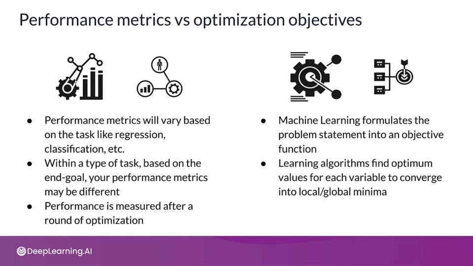
Performance metrics vs optimization objectives

tion="Source: https://cs231n.github.io/neural-networks-3/">}}

The above gif shows different optimization function finding to optima value for loss function, on loss surface.

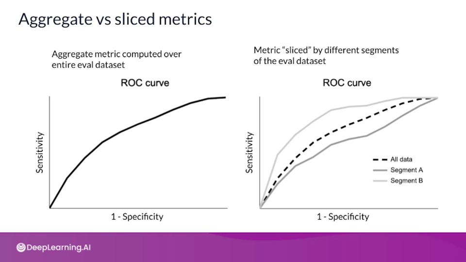
Top level aggregate metrics vs slicing

Most of the time, metrics are calculated on the entire dataset
Slicing deals with understanding how the model is performing on each subset of data.

TensorBoard

If you wish to dive more deeply into TensorBoard usage for model analysis feel free to check out this optional reference. You won’t have to read these to complete this week’s practice quizzes.

TensorBoard

Advanced Model Analysis and Debugging — Introduction to TensorFlow model Analysis (TFMA)

Why should you slice your data?

Your top-level metrics may hide problems

Your model may not perform well for particular [customers | products | stores | days of the week | etc.]

Each prediction request is an individual event, maybe an individual customer

For example, customers may have a bad experience
For example, some stores may perform badly

TensorFlow Model Analysis (TFMA)

TFMA is a open source, scalable, and a versatile tool for doing deep analysis of your model's performance.

Ensure models meet required quality thresholds
Used to compute and visualize evaluation metrics
Inspect model's performance against different slices of data

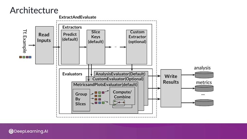
Architecture

The first stage Read inputs is made up of transform that takes raw input and converts into a dictionary format , tfma.Extracts to be understandable by next stage 'Extraction'. Across all stages the output is kept in this dictionary format.
The next stage Extraction performs distributed processing using Apache Beam. Input extractor and slice key extractor forms slices of the original dataset, which will then be utilized by predict extractor to run predictions on each slice.
The next stage Evaluation also performs distributed processing using Apache Beam. We can even create custom evaluator.
The final stage Write Results writes the result to disk.

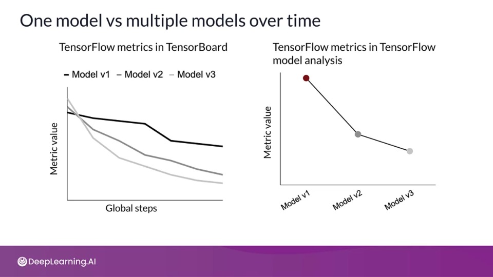
One model vs multiple models over time

TensorBoard visualizes streaming metrics of multiple models over global training set.

TFMA visualizes the metrics computes across different saved model versions

Aggregate vs sliced metrics

Determining which slices are important to analyze requires domain knowledge about the data and application.

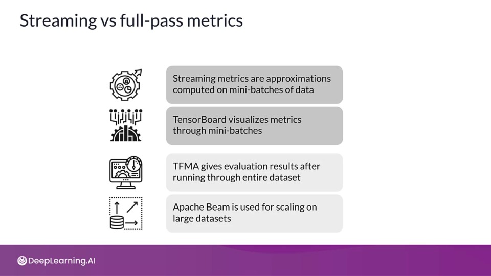
Streaming vs full-pass metrics

TFMA in Practice

Analyze impact of different slices of data over various metrics
How to track metrics over time?
When you use TFMA in a TFX pipeline, the evaluator component already contains many of the steps described here.

Step 1: Export EvalSavedModel for TFMA

import tensorflow as tf
import tensorflow_transform as tft
import tensorflow_model_analysis as tfma

def get_serve_tf_examples_fn(model, tf_transform_output):
    # Return a function that parses a serialized tf.Example and applies TFT
    tf_transform_output = tft.TFTransformOutput(transform_output_dir)

signatures = {
    'serving_default': get_serve_tf_examples_fn(model, tf_transform_output)
                                                                                            .get_concreate_function(tf.TensroSpec(...)),
}
model.save(serving_model_dir_path, sava_format='tf', signatures=signatures)

Step 2: Create EvalConfig

Create eval_config object that encapsulates the requirements for TFMA.

# Specify slicing spec
slice_spec = [slicer.SingleSliceSpec(columns=['column_name']), ...]

# Define metrics
metrics = [tf.keras.metrics.Accuracy(name='accuracy'),
                     tfma.metrics.MeanPrediction(name='mean_prediction'),
           ...]
metrics_specs = tfma.metrics.specs_from_metrics(metrics)

eval_config = tfma.EvalConfig(
                                     model_specs=[tfma.ModelSpec(label_key=features.LABEL_KEY)],
                                     slicing_specs=slice_spec,
                                     metrics_specs=metrics_specs,
                   ...)

Step 3: Analyze model

# Specify the path to the eval graph and to where the result should be written
eval_model_dir = ...
result_path = ...

eval_shared_model = tfma.default_eval_shared_model(
                                                        eval_saved_model_path=eval_model_dir,
                                                        eval_config=eval_config)

# RUN TensorFlow Model Analysis
eval_result = tfma.run_model_analysis(eval_shared_model=eval_shared_model,

Step 4: Visualizing metrics

# rendder results
tfma.viewer.render_slicing_metrics(result)

TensorFlow Model Analysis

If you wish to dive more deeply into TensorFlow Model Analysis (TFMA) capabilities, feel free to check out these resources. You won’t have to read these to complete this week’s practice quizzes.

Model Debugging Overview

Model robustness

Robustness is much more than generalization
Is the model accurate even for slightly corrupted input data?

Robustness metrics

Robustness measurement shouldn't take place during training and not using training data
Split data into train/val/test sets
Specific metrics for regression and classification problems

Model Debugging

Deals with detecting and dealing with problems in ML systems
Applies mainstream software engineering practices to ML models

Objectives:

Opaqueness

Model debugging tries to improve the transparency of models by highlighting how data is flowing inside.
Social discrimination

Model shouldn't work poorly for certain groups of people.
Security vulnerabilities

Model debugging also aims to reduce the vulnerability of your model to attacks.
Privacy harms

The data should be anonamized before training
Model decay

Model performance decays with time as the distribution of incoming data changes.

Model Debugging Techniques

Benchmark models
Sensitivity analysis
Residual analysis

Benchmark Models

Benchmarking model are simple but consistence performance giving models that are used before you start development for baselining your problem.

Compare your model against these models to see if its performing better than the simpler benchmarking model as a sanity test.

Once the model passes the benchmark test, the benchmark model become a solid debugging tool and a starting point of ML development.

Sensitivity Analysis and Adversarial Attacks

Sensitivity analysis helps us understand the model by examining the impact each feature has on the model's prediction.

In sensitivity analysis we experiment by changing a single feature's value while holding the other features constant and observe the model results.

If changing the features values causes the models result to be drastically different. It means that that feature has a big impact on the prediction.

See how model reacts to data which has never been used before
What-If tool developed by TensorFlow team allows to perform sensitivity analysis to understand and debug you model performance.

Common approaches for doing sensitivity analysis:

1. Random Attacks

Expose models to high volumes of random input data.
Exploits the unexpected software and math bugs
Great way to start debugging

2. Partial dependence plots

Partial dependence plots show the marginal effect of one or two features and the effect they have on the model results.
These plots can describe the relationship between outcome and a particular feature is linear, monotonic or more complex.
PDPbox and PyCEbox are open source packages for creating such plots.

How vulnerable to attacks is your model?

Sensitivity can mean vulnerability

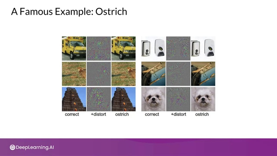
Attacks are aimed at fooling your model by creating examples which are formed by making small but carefully designed changes to the data.
Successful attacks could be catastrophic
Test adversarial examples
Harden your model

Informational and Behavioral Harms

Informational Harm: unanticipated leakage of information
Behavioral Harm: manipulating the behavior of the model

Informational Harms

Membership Inference attacks: was this person's data used for training?

These attacks are aimed at inferring whether or not an individual's data was used to train the model based on a sample of the model's output
Model Inversion attacks: recreate the training data
Model Extraction: recreate the model

Behavioral Harms

Poisoning attacks: insert malicious data into training data in order to change the behavior of the model.
Evasion attacks: input data that causes the mode to intentionally misclassify that data

Measuring your vulnerability to attack

Cleverhans: an open-source Python library to benchmark machine learning systems's vulnerability to adversarial examples.

To harden your model to adversarial attacks, one approach is to include adversarial examples into the training set, this is referred to as adversarial training.

Foolbox: an open-source Python library that lets you easily run adversarial attacks against machine learning models.

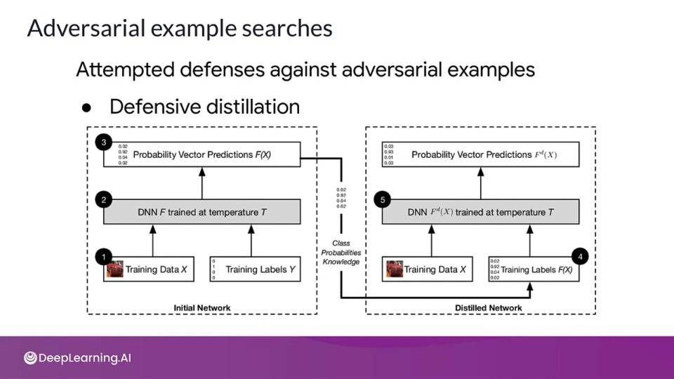
Adversarial example searches

Attempted defenses against adversarial examples:

Defensive distillation: the main difference from the original distillation is that we use the same architecture to train both the original network as well as the distilled network.

Sensitivity Analysis and Residual attacks

If you wish to dive more deeply into adversarial attacks, feel free to check out this paper:

Explaining and Harnessing Adversarial Examples

To access the Partial Dependence Plots libraries please check these resources:

The demo shown in the previous video is based on this Google Colab notebook.

Residual Analysis

Measures the differences between model's performance and ground truth
Randomly distributed errors are good
Correlated or systematic errors show that a model can be improved

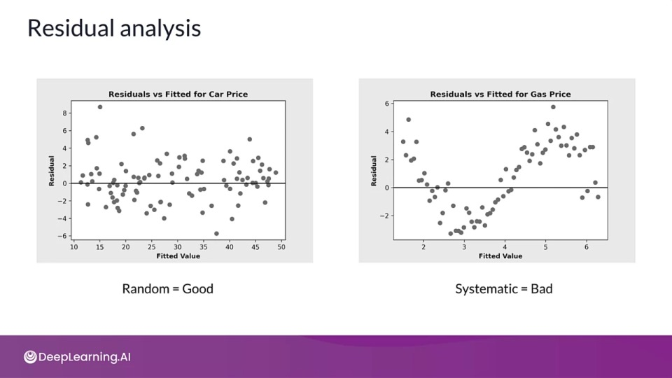
Residuals should not be correlated with another feature
Adjacent residuals should not be correlated with each other (autocorrelation)

Performing a Durbin Watson test is also useful for detecting autocorrelation.

Model Remediation — How to improve robustness?

Data augmentation:

Adding synthetic data into training set
Helps correct for unbalanced training data

Interpretable and explainable ML:

Understand how data is getting transformed
Overcome myth of neural networks as black box

Model editing:

Applies to decision trees
Manual tweaks to adapt your use case

Model assertions:

Implement business rules that override model predictions

Reducing or eliminating Model Biaas

Discrimination remediation

Include people with varied backgrounds for collecting training data
Conduct feature selection on training data
Use fairness metrics to select hyperparameters and decision cut-off thresholds

Remediation in production

Model monitoring

Conduct model debugging at regular intervals
Inspect accuracy, fairness, security problems, etc.

Anomaly detection

Anomalies can be a warning of an attack
Enforce data integrity constraints on incoming data

Fairness

Make sure model does not cause harm to specific group of people

Fairness indicators is an open source library to compute fairness metrics
Easily scales across dataset of any size
Built on top of TFMA

What does fairness indicators do?

Compute commonly-identified fairness metrics for classification models
Compare model performance across subgroups to other models
No remediation tools provided

Evaluate at individual slices

Overall metrics can hide poor performance for certain parts of data
Some metrics may fare well over others

Aspects to consider

Establish context and different user types
Seek domain experts help
Use data slicing widely and wisely

General guidelines

Compute performance metrics at all slices of data
Evaluate your metrics across multiple thresholds
If decision margin is small, report in more detail

Measuring Fairness

Positive rate / Negative rate

Percentage data points classified as positive/negative
Independent of ground truth
Use case: having equal final percentages of groups is important

True positive rate (TPR) / False negative rate (FNR)

TPR: percentage of positive data points that are correctly labeled positive

FNR: percentage of positive data points that are incorrectly labeled negative

Measures equality of opportunity, when the positive class should be equal across subgroups
Use case: where it is important that same percent of qualified candidates are rated positive in each group

False Positive rate (FPR) / True negative rate (TNR)

FPR: percentage of negative data points that are incorrectly labeled negative.

TNR: percentage of negative data points that are correctly labeled negative

Measures equality of opportunity, when the negative class should be equal across subgroups
Use case: where misclassifying something as positive are more concerning than classifying the positives.

Accuracy & Area under the curve (AUC)

Accuracy: percentage of data points that are correctly labeled

AUC: percentage of data points that are correctly labeled when each class is given equal weight independent of number of samples

Metrics related to predictive parity
Use case: when precision is critical

Some Tips

Unfair skews if there is a gap in a metric between two groups
Good fairness indicators doesn't always mean the model is fair
Continuous evaluation throughout development and deployment
Conduct adversarial testing for rare, malicious examples
Model Remediation and Fairness

Model Remediation and Fairness

If you wish to dive more deeply into model remediation and fairness, feel free to check out these optional resources and tools. You won’t have to read these to complete this week’s practice quizzes.

Continuous Evaluation and Monitoring

Why do models need to be monitored?

Training data is a snapshot of the world at a point in time
many types of data change over times, some quickly
ML Models do not get better with age
As model performance degrades, you want an early warning

Data drift and shift

Concept drift: change in the relationship between inputs and labels.

Concept Emergence: new type of data distribution

Types of dataset shift:

Covariate shift: The distribution of your input data changes but the conditional probability of your output over the input remains the same. Distribution of label doesn't change.
Prior probability shift: The distribution of your labels changes but the input data remains same.

Concept drift can be taught of as a type of prior probability shift.

How do you find the shift and drift. There are both supervised and unsupervised techniques. Let's discuss them:

Statistical process control — supervised

Method used: drift detection method

It assumes that the stream of data will be stationary and then models the number of errors as binomial random variable

$$ \mu = np_t \qquad \sigma = \sqrt{\frac{p_t(1-p_t)}{n}} $$

Alert rule

$$ p_t + \sigma_t \geq p_{min} + 3\sigma_{min} \implies \text{ALERT!} $$

Analyses the rate of errors and since it's a supervised method it requires us to have labels for incoming stream of data. It triggers a drift alert if the parameters of the distributions go beyond a certain thresholds.

Sequential analysis — supervised

Method used: Linear four rates

The idea is if data is stationary, continency table should remain constant
The contingency table here corresponds to the truth table for a classifier

We calculate four rates:

$$ P_{npv} = \frac{TN}{TN+FN} \quad P_{precision} =\frac{TP}{TP+ FP} \\[10pt] P_{recall / sensitivity / TPR} = \frac{TP}{TP+FN}\quad P_{specificity/ FPR} = \frac{TN}{TN+FP} \\[10pt] P_*^t \leftarrow \eta_*P_*^{t-1} + (1-\eta_*) I_{y_t=\hat{y}_t} $$

If model is predicting correctly, these four values remain constant.

Error distribution monitoring — unsupervised

Method used: Adaptive Windowing (ADWIN)

In this method you divide the incoming data into windows. Calculate mean error rate at every window of data.
Size of window adapts, becoming shorter when data is not stationary

Calculate absolute of mean error rate at every successive window and compare it with threshold based on the Hoeffding bound.

$$ |\mu_0 -\mu_1| > \Theta_\text{Hoeffding} $$

The Hoeffding bound is used for testing the difference between the means of two populations.

Clustering/novelty detection — unsupervised

Assign data to known cluster or detect emerging concept

Multiple algorithms available: OLINDDA, MINAS, ECSMiner, and GC3, etc.
Susceptible to curse of dimensionality
Can only detect cluster based drift not detect population based changes

Feature distribution monitoring — unsupervised

Monitors individual feature separately at every window of data, comparing individual features against each window of data.

Algorithms to compare:

Pearson correlation in Change of Concept
Hellinger Distance in HDDDM (Hellinger Distance Drift Detection Method)

Use PCA to reduce number of features

Cannot detect population drift since it looks only at individual features

Model-dependent monitoring — unsupervised

This method monitors the space near the decision boundaries or margins in the latent feature space of your model.

one algorithm is Margin Density Drift Detection (MD3)
Area in latent space where classifier have low confidence matter more
- A change in the number of samples in the margin, margin density indicates drift
Reduce false alarm rate

Google Cloud AI Continuous Evaluation

Leverages AI Platform Prediction and Data Labeling services
Deploy your model to AI Platform Prediction with model version
Create evaluation job
Input and output are saved in BigQuery table
Run evaluation job on a few of these samples
View the evaluation metrics on Google Cloud console

How often should you retrain?

Depends on the rate of change
If possible, automate the management of detecting model drift and triggering model retraining.

Continuous Evaluation and Monitoring

If you wish to dive more deeply into continuous evaluation and model monitoring, feel free to check out these optional resources and tools. You won’t have to read these to complete this week’s practice quizzes.