Week 2 — Basics of Neural Network programming
May 1, 2021
Logistic Regression as a Neural Network
- Logistic Regression is an algorithm for Binary Classification.
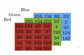
Consider we have an image we want to classify as cat or not of 64x64 dimension
-
The images are stored as matrix pixel intensity value for different color channels. (one matrix per color channel and with each layer dimension being the dimension of image).
To represent image we can use a single feature vector:
So $n_x$ (input size) becomes $64\times64\times3 = 122288$.
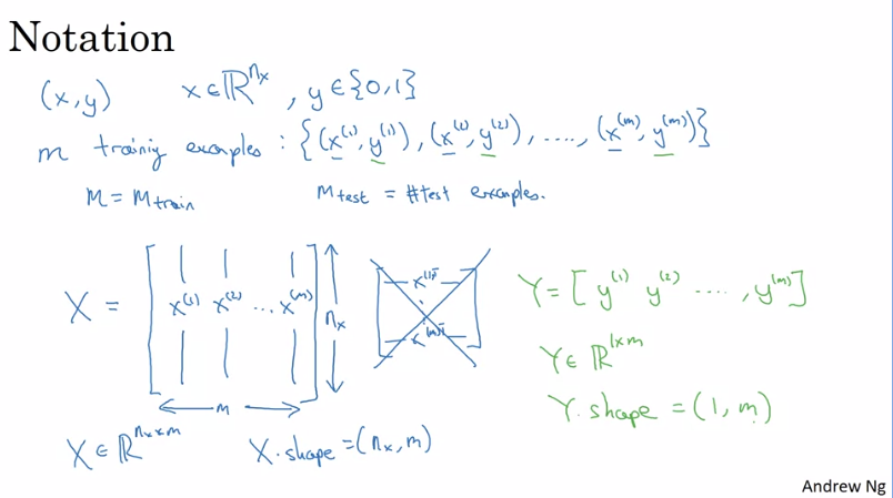
Notations:
Logistic Regression
In formal terms for cat classification problem:
Given $x$, want $\hat{y} = \text{P}(y=1|x)$.
where,
- $x \in \mathbb{R}^{n_x}$
Parameters: $w\in \mathbb{R}^{n_x}, b\in \mathbb{R}$
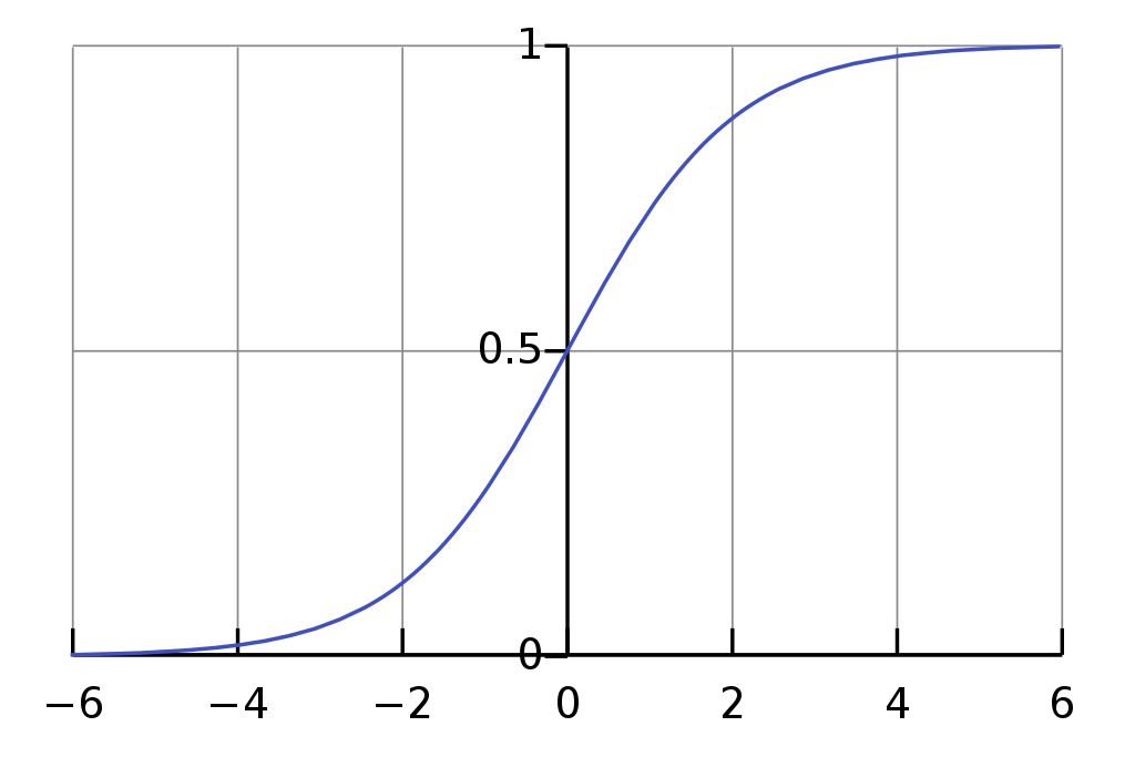
Output or Activation function
Output : $\hat{y} = \sigma(w^\intercal x + b)$
where,

Hence, this satisfy the two conditions:dx
If $z$ is large:
$$ \sigma(z) \approx \frac{1}{1+0} = 1 $$
If z is large negative number then, the exponential function returns very big value.
$$ \sigma(z) \approx \frac{1}{1+bigno} \approx 0 $$
Warning
In a alternate notation you might see (like in Hands-on machine learning book) $\hat{y} = \sigma(x^{\intercal}\theta)$ instead of $\sigma(w^\intercal x + b)$. In this notation $\theta_0$ represent bias vector and rest of the $\theta$ vector contains the weights.
But in this course we will not be using this convention.
Logistic Regression Cost Function
- Cost function (loss function for single training example) to optimize, want to be as small as possible.The Loss function is cost function averaged for all training instances.
$$ J(w, b)=J(\theta) = -\frac{1}{m}\sum^m_{i=1}\bigg[y^{(i)}\log\Big(\hat{y}^{(i)}\Big)+ \Big(1-y^{(i)}\Big)\log\Big(1-\hat{y}^{(i)}\Big)\bigg] $$
- The cost function for single training example, we want:
- That means
- If label is 1, we want $(-\log(\hat{y}))$ to be as small as possible $\rightarrow$ want $(\log\hat{y})$ to be large as possible $\rightarrow$ want $\hat{y}$ to be large (i.e. $\approx 1$).
- If label is 0, we want $(-\log(1- \hat{y}))$ to be as small as possible $\rightarrow$ want $(\log1-\hat{y})$ to be large $\rightarrow$ want $\hat{y}$ to be small.
Gradient Descent
May 2, 2021
Gradient Descent is a generic optimization algorithm capable of finding optimal solutions to a wide range of problems, The general idea of Gradient Descent is to tweak parameters iteratively to minimize cost function.
We have a cost function for logistic regression.
$$ J(w, b)=J(\theta) = -\frac{1}{m}\sum^m_{i=1}\bigg[y^{(i)}\log\Big(\hat{y}^{(i)}\Big)+ \Big(1-y^{(i)}\Big)\log\Big(1-\hat{y}^{(i)}\Big)\bigg] $$
Where.
- $\alpha$ is a hyperparmeter for learning rate.
- Derivative tells the slope of the function OR how a small change in a value what change comes to the function.
- On the left side the derivative (slope) will be negative making us increasing the weights.
- On the right side the derivative (slope) will be positive which will result in decreasing the weights.
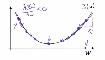
- So we will update the weights and bias like this:
$$ w = w - \alpha\frac{\partial J(w,b)}{\partial w} $$
$$ b = b - \alpha \frac{\partial J(w, b)}{\partial b} $$
Tip
Remember $d$ is used for derivative whereas $\partial$ is used to denote partial derivative when the function we want to derivate has multiple other variables (which are considered constant at the time we are finding the derivative).
Derivatives
Computation Graph
A computational graph is defined as a directed graph where the nodes correspond to mathematical operations. Computational graphs are a way of expressing and evaluating a mathematical expression.
- The computation graph explains why the computations of neural network is organised with first a forward pass and then a backward pass in Backpropagation algorithm.
- Reverse-mode autodiff performs a forward pass through a computation graph, computing every node's value for the current training batch, and then it performs a reverse pass, computing all the gradients at once.
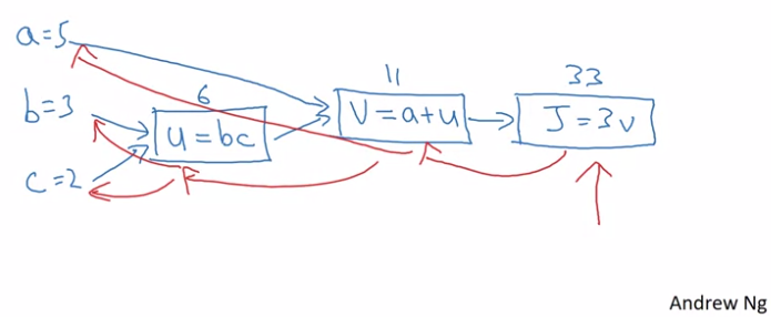
- Let's say we have a function
$$ J(a, b, c) = 3(a + bc) $$
- In this we have 3 steps (represented by nodes) to compute. These are:
$u = bc$
$v = a+u$
$J = 3v$
Computing with a computation Graph
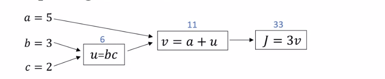
- Let's say we want to compute the derivative of $J$ with respect to $v$. $\frac{dJ}{dv} = ?$
- i.e. for a little change in $v$ how the value of $J$ changes?
- We know from our calculus class, the derivative should be:
$$ \frac{dJ}{dv} = \bold{3} $$
- Then we want to compute the derivative of $J$ with respect to $a$. We can use chain rule which says:
If $a$ affects $v$ affects $J$ ($a \rightarrow v \rightarrow J$) then the amounts that $J$ changes when you nudge $a$ is the product of how much $v$ changes when you nudge $a$ times how much $J$ changes when you nudge $v$.
$$ \frac{dv}{da} = \bold{1} \ [10pt] \frac{dJ}{da} = \frac{dJ}{dv}\frac{dv}{da} = 3 \times 1 = \bold{3} $$
- This illustrates how computing $$\frac{dJ}{dv}$$ let's us compute $$\frac{dJ}{da}$$.
- In the code we will be using
dvarto represent the the derivative of the final output variable with respect to any variablevar. - Let's do it for other variables.
- What is the derivative of $J$ with respect to $u$.
$$ \frac{dJ}{du} = \frac{dJ}{dv}\frac{dv}{du} = 3 \times 1 = \bold{3} $$
- And then derivative of $J$ with respect to $b$
$$ \frac{du}{db} = 2 $$
$$ \frac{dJ}{db} = \frac{dJ}{du}\frac{du}{db} = 3 \times 2 = \bold{6} $$
- The derivative of $J$ with respect to $c$
$$ \frac{dJ}{dc} = \frac{dJ}{du}\frac{du}{dc} = 3 \times 3 = \bold{9} $$
Gradient Descent for Logistic Regression
- Logistic regression recap
$z = w^\intercal +b$
$\hat{y} = \hat{p} = \sigma(z)$
$L(\hat{y}, y) = - \Big[y\log (a) + (1-y)\log(1-\hat{y})\Big]$
- Let's say we have only two features, then we will have two weight and a bias.
The computation graph
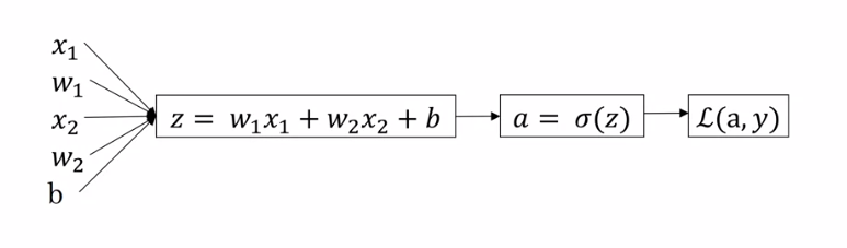
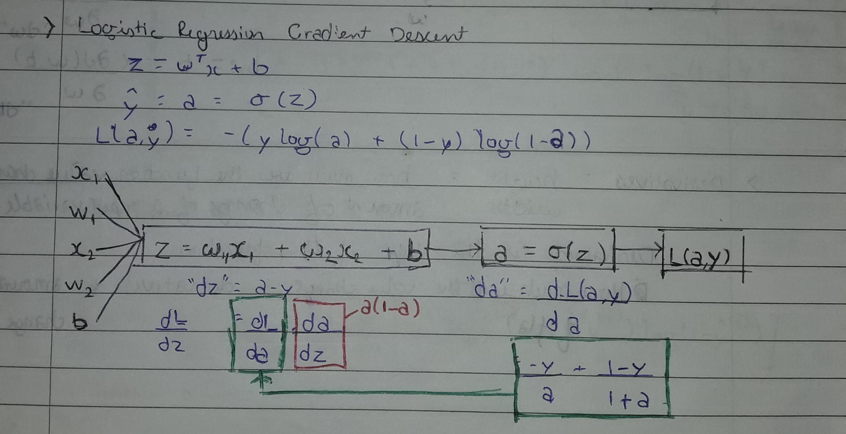
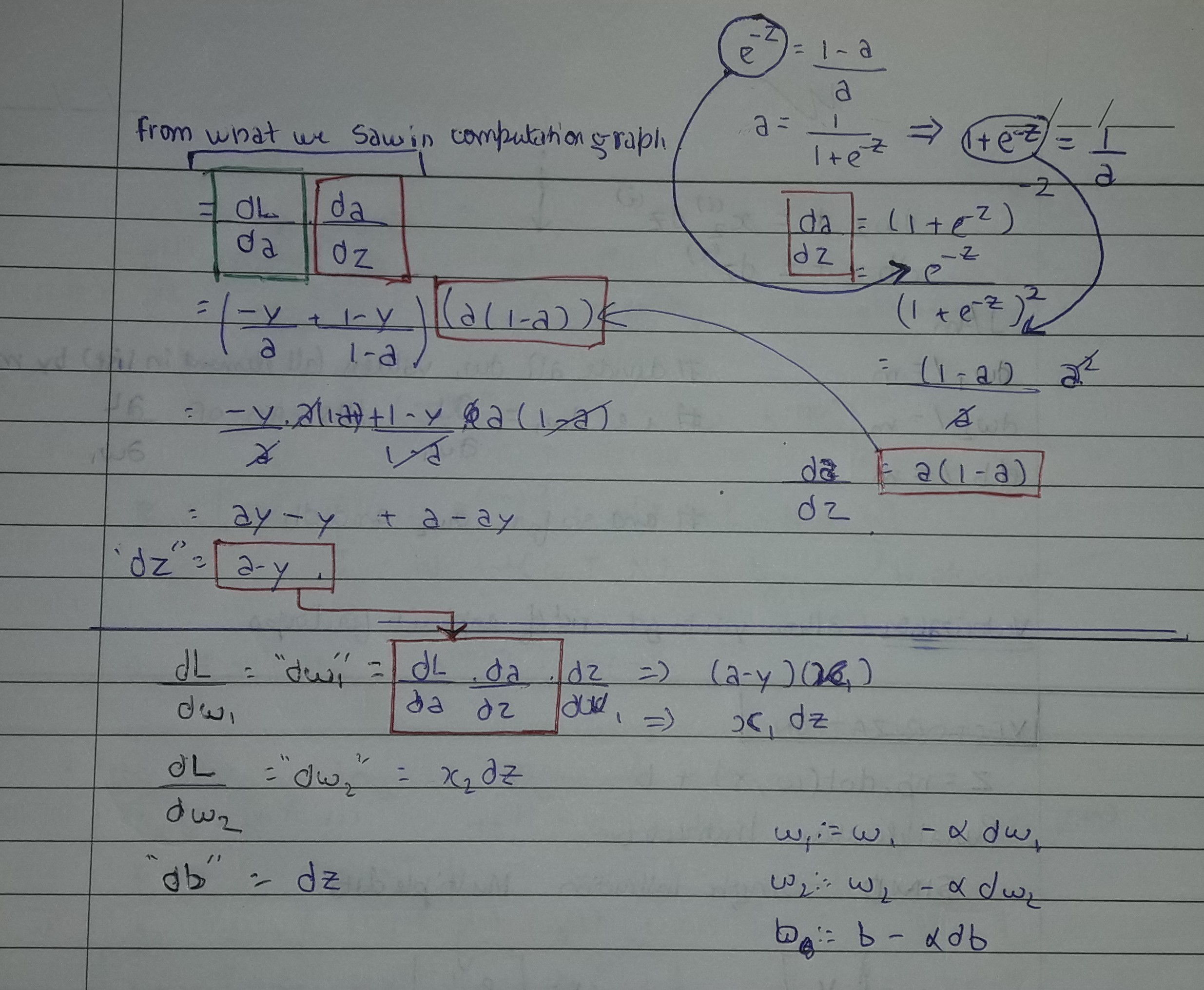
Hence, we use $dz = (a-y)$ for calculating Loss function for single instance with respect to $w_1$ by calulating:
$$ \frac{dL}{dw_1} = \frac{dL}{da}\frac{da}{dz}\frac{dz}{dw_1} = (a-y)(x_1) = \bold{x_1\frac{dL}{dz}} $$
and with respect to $w_2$
$$ \frac{dL}{dw_2} = \frac{dL}{da}\frac{da}{dz}\frac{dz}{dw_2} = (a-y)(x_2) = \bold{x_2\frac{dL}{dz}} $$
for bias it remains same:
$$ \frac{dL}{db} = \bold{\frac{dL}{dz}} $$
This makes the updates like this:
$$ w_1 = w_1 - \alpha dw_1\\ w_2 = w_2 = \alpha dw_2\\b = b -\alpha db $$
- where $dw_1, dw_2, db$ as said earlier represents the derivative of the final output variable (Loss function) with respect to respective variable.
Gradient Descent on $m$ Examples
This Loss function is for $m$ training examples computed over $(i)^\text{th}$ instances.
$$ J(w, b)=J(\theta) = -\frac{1}{m}\sum^m_{i=1}\bigg[y^{(i)}\log\Big(\hat{y}^{(i)}\Big)+ \Big(1-y^{(i)}\Big)\log\Big(1-\hat{y}^{(i)}\Big)\bigg] $$
- where $$\hat{y} = \sigma(z^{(i)}) = \sigma(w^\intercal x^{(i)} + b)$$ is the prediction over one training example.
So for calculating Cost function derivative with respect to first weight becomes:
$$ \frac{\partial J}{\partial w_1} = \frac{1}{m}\sum^m_{i=1} \frac{\partial}{\partial w_1}L(\hat{y}^{(i)}, y^{(i)}) $$
Which as we have seen will then be:
$$ \frac{\partial J}{\partial w_1} = \frac{1}{m}\sum^m_{i=1} dw_1^{(i)} \qquad\qquad \frac{\partial J}{\partial w_2} = \frac{1}{m}\sum^m_{i=1} dw_2^{(i)} $$
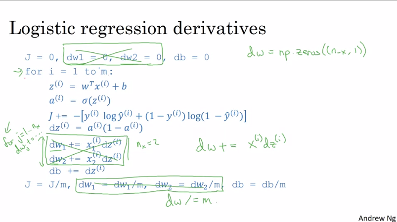
Wrap up in algorithm (what we can do)
Assuming we have only two features. The single step of gradient descent will look like:
$j=0,\; dw_1=0,\; dw_2=0,\; db=0\\\text{For} \enspace i=1\enspace\text{to}\enspace m:$
$\qquad z^{(i)} = w^\intercal x^{(i)} + b\\\qquad \hat{y}^{(i)} = \sigma(z^{(i)})\\\qquad J \enspace+= -\Big[y^{(i)}\log\hat{y}^{(i)}+ \big(1-y^{(i)}\big)\log\big(1-\hat{y}^{(i)}\big)]\\\qquad dz^{(i)} = \hat{y}^{(i)} - y^{(i)}\\\qquad dw_1\enspace += x_1^{(i)}dz^{(i)}\enspace\fcolorbox{red}{white}{here $dw_1$ is used as accumulator}\\\qquad dw_2 \enspace += x_2^{(i)}dz^{(i)}\enspace\fcolorbox{red}{white}{h ere $dw_2$ is used as accumulator}\\\qquad db\enspace+= dz^{(i)}$
$J \enspace/=m \qquad\fcolorbox{red}{white}{averaging cost function over $m$ training examples}\\dw_1\enspace /=m; \; dw_2\enspace/=m\; db\enspace/=m\\w_1 = w_1 - \alpha dw_1\\ w_2 = w_2 = \alpha dw_2\\b = b -\alpha db$
- We have a problem here in which we require two for loops:
- One for iterating over $m$ training example.
- another one iterating over feature set calculating the derivative per feature.
Vectorization
Whenever possible, avoid explicit for-loops. Use vectorization.
Vectorization relies on parallelization instructions called SIMD (Single Instruction Multiple Data), which can be be found in both CPU and GPU but GPUs are better at that.
IMPORTANT
Andrew refers to $dz = a (1-a)$
Note that Andrew is using "$dz$" as a shorthand to refer to $\frac{da}{dz} = a (1-a)$ .
Earlier in this week's videos, Andrew used the name "$dz$" to refer to a different derivative: $\frac{dL}{dz} = a -y$.
Note: here $a$ is $\hat{y}$
Vectorizing Logistic Regression
We can make the prediction or the forward propagation step like this:
Step 1
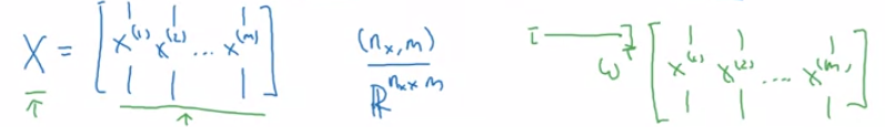
$$ Z = [z^{(i)}, z^{(2)}, ..., z^{(m)}]= w^\intercal X + [b, b, b, ....b] $$
where,
- $X$ represent the $(n_x, m)$ dimensional feature matrix.
- $[b, b, b, ....b]$ is bias matrix with $(1, m)$ dimension.
In Python
Step 2
$$ \hat{Y} = [\hat{y}^{(1)}, \hat{y}^{(2)}, ..., \hat{y}^{(m)}] = \sigma(Z) $$
Vectorizing Logistic Regression's Gradient Output
vectorizing calculation of "dz" ($\frac{dL}{dz}$)
We want: $dz^{(1)} = [\hat{y}^{(1)} - y^{(1)}]$, $dz^{(2)}= [\hat{y}^{(2)} - y^{(2)}]$,...
$dZ = [dz^{(1)}, dz^{(2)}, ..., dz^{(m)}]$
Then:
$\hat{Y} = [\hat{y}^{(1)}, ..., \hat{(m)}]$ $Y = [y^{(1)},..., y^{(m)}]$
$dZ = \hat{Y} - Y$
vectorizing updates of weights and bias
$dw = \frac{1}{m}X{dZ}^\intercal$
Which creates as ($n, 1$) dimensional vector with each element being from $dz_{(i)}$ to $dz_{(n)}$ where $n$ is the number of features.
$db = \frac{1}{m} \sum^m_{i=1} dz^{(i)}$
which in python is done using
Implementing Logistic Regression
$Z = w^\intercal X +b = \text{np.dot(w.T, X)+b}$
$\hat{Y} = \sigma(Z) $
$dZ = \hat{Y} - Y$
$dw= \frac{1}{m}XdZ^\intercal$
$db = \frac{1}{m}\text{ * np.sum($dZ$)}$
$w = w -\alpha dw$
$b = b - \alpha db$
General Principle of Broadcasting
If we have $(m, n)$ matrix and for any operation we want to do with $(1, n)$ or $(m, 1)$ matrix, the matrix with be converted to $(m, n)$ dimensional matrix by copying.
If we have $(m, 1)$ or $(1, m)$ matrix and for any operation we want to do with a real number $R$ get converted to $(m, 1)$ or $(1, m)$ dimensional matrix by copying $R$.
A note on python/NumPy vectors
import numpy as np

a = np.random.randn(5)
print(a)
>>> [0.502, -0.296, 0.954, -0.821, -1.462]

print(a.shape)
>>>(5,)
Vectors like a are called rank 1 array in python. That is it is neither a row vector, nor a column vector. Which leads to some slightly non-intuitive effects such as-
print(a.T)
>>> [0.502, -0.296, 0.954, -0.821, -1.462]

print(np.dot(a, a.T)   # should probanly be matrix product
>>>  4.06570109321
Instead do this:
If you get a rank 1 array, just reshape it.
Some important Points
- Softmax function
$$ \text{for a matrix } x \in \mathbb{R}^{m \times n} \text{, $x_{ij}$ maps to the element in the $i^{th}$ row and $j^{th}$ column of $x$, thus we have: } $$
- L1 loss is defined as:
$$ \begin{align*} & L_1(\hat{y}, y) = \sum_{i=0}^m|y^{(i)} - \hat{y}^{(i)}| \end{align*}\tag{1} $$
- L2 loss is defined as:
$$ \begin{align*} & L_2(\hat{y},y) = \sum_{i=0}^m(y^{(i)} - \hat{y}^{(i)})^2 \end{align*}\tag{2} $$
A trick when you want to flatten a matrix $X$ of shape $(a,b,c,d)$ to a matrix $X_flatten$ of shape $(b∗c∗d, a)$ is to use: