Week 2 — Dimensionality Reduction
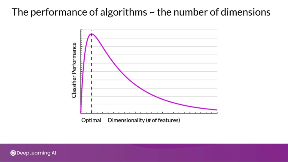
Dimensionality Effect on Performance
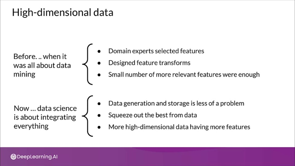
A note about neural networks
- Yes, neural networks will perform a kind of automatic feature selection
- However, that's not as efficient as a well-designed dataset and model
- Much of the model can be largely "shut off" to ignore unwanted features
- Even unused parts of the model consume space and compute resources
- Unwanted features can still introduce unwanted noise
- Each feature requires infrastructure to collect, store, and manage.
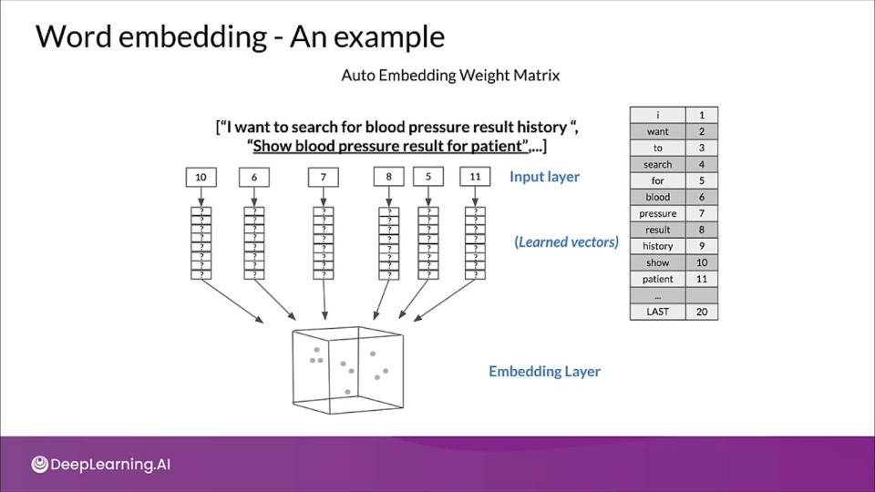
# WORD EMBEDDING EXAMPLE

import tensorflow as tf
from tensorflow import keras
import numpy as np
from keras.datasets import reuters
from keras.preprocessing import sequence

NUM_WORDS = 1_000 # Least repeated words are considered unknown

(reuters_train_x, reuters_train_y), (reuters_test_x, reuters_test_y) =
  tf.keras.dataset.reuters.load_data(num_words=NUM_WORDS)
n_laberls = np.unique(reuters_train_y).shape[0]

# Further preprocessing
from keras.utils import np_utils
reuters_train_y = np_utils.to_categorical(reuters_train_y, 46)
reuters_test_y = np_utils.to_categorical(reuters_test_y, 46)

reuters_train_x = keras.preprocessing.sequence.pad_sequence(
  reuters_train_x, maxlen=20)
reuters_test_x = keras.preprocessing.sequence.pad_sequence(
  reuters_test_x, maxlen=20)

# Using all dimensions
from tensorflow.keras import layers
model = keras.Sequential([
    # The embedding is projected to 1000 dimesions here (2nd parameter)
    layers.Embedding(NUM_WORDS, 1000, input_length=20),
    layers.Flatten(),
    layers.Dense(256),
    layers.Dropout(0.25),
    layers.Actiation('relu'),
    layers.Dense(46),
    layers.Activation('softmax')
])

# Model compilation and training
model.compile(loss='categorical_crossentropy',
              optimizer='rmsprop',
              metrics=['accuracy'])

model_1 = model.fit(reuters_train_x, reuters_train_y,
                    validation_data=(reuters_test_x
                    reuters_test_y),
  batch_size=128, epochs=20, verbose=0)
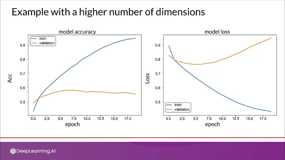 tion="This model is overfitting as the model clearly perform poorly on validation set, and a high loss for validation set compared to training loss." >}}
Word embeddings: 6 dimensions instead of 1000
 model = keras.Sequential([
    # The embedding is projected to 1000 dimesions here (2nd parameter)
    layers.Embedding(NUM_WORDS, 6, input_length=20),
    layers.Flatten(),
    layers.Dense(256),
    layers.Dropout(0.25),
    layers.Actiation('relu'),
    layers.Dense(46),
    layers.Activation('softmax')
])
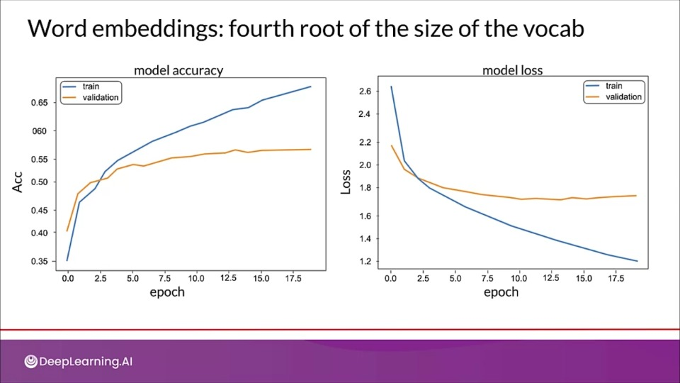 tion="Although there is some overfitting, The newer model seems to perform better" >}}
Curse of Dimensionality
Many ML methods use the distance measures like KNN, SVM and recommendation systems.
Most common being Euclidean Distance.
Why is high-dimensional data a problem?
- More dimension $\rightarrow$ more features
- Risk of overfitting our models
- Distances grow more and more alike, vectors might appear equidistant from all others.
- No clear distinction between clustered objects
- Concentration phenomenon for Euclidean distance
- Distribution of norms (distance between vectors) in a given distribution of points tends to concentrate.
- Adding dimensions increases feature space volume
- Solutions take longer to converge, might get stuck in local optima
- Runtime and system memory requirements
Why are more features bad?
- Redundant/irrelevant features
- More noise added than signal
- Hard to interpret and visualize
- Hard to store and process data
Curse of dimensionality in the distance function
$$ d_{i,j} = \sqrt{\sum_{k=1}^n(x_{ik} - x_{jk})^2} \tag{Euclidean distance} $$
- New dimensions add non-negative terms to the sum
- Distance increases with the number of dimensions
- For a given number of examples, the feature space becomes increasingly sparse
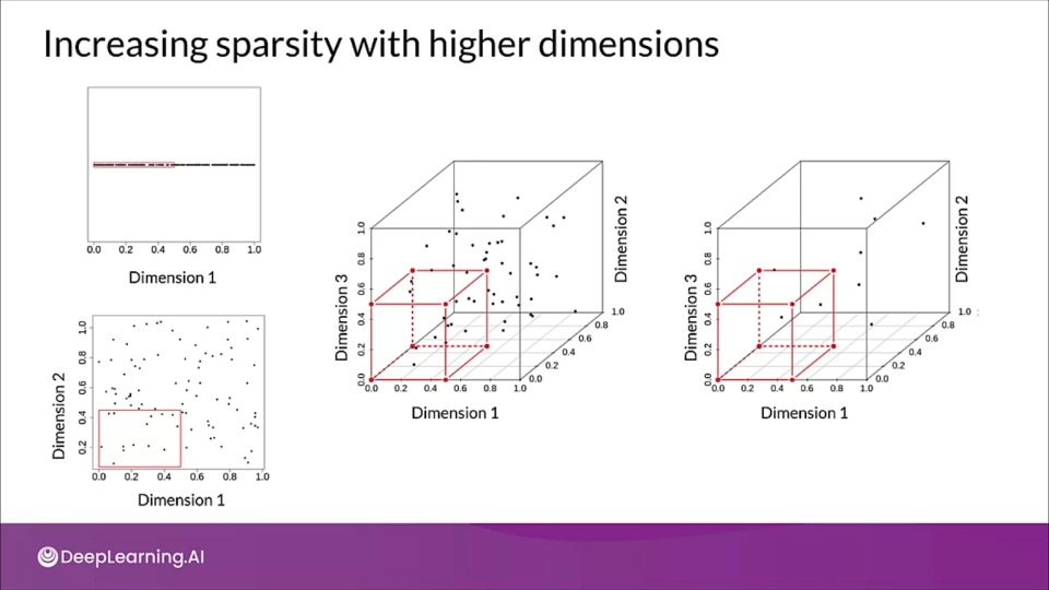
- The size of the feature space grows exponentially as the number of features increases making it much harder to generalize efficiently.
- The variance increases, features might even be correlated and thus there are higher chances of overfitting to noise.
- The challenge is to keep as much of the predictive information as possible using as few features as possible.
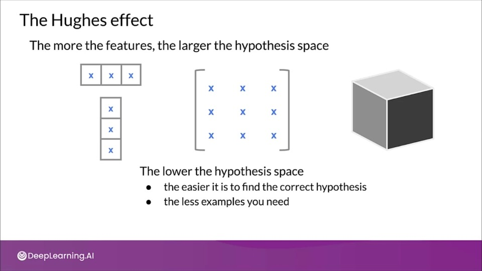
The Hughes effect
The more the features, the large the hypothesis space.
Curse of Dimensionality: an Example
- More features aren't better if they don't add predictive information
- Number of training instances needed increases exponentially with each added feature
What do ML models need?
- No hard and fast rule on how many features are required
- Number of features to be used vary depending on the amount of training data available, the variance in that data, the complexity of the decision surface, and the type of classifier that is used. It can also depend on which features actually contain predictive information.
- Prefer uncorrelated data, with containing predictive information to produce correct results
Manual Dimensionality Reduction
Increasing predictive performance
- Features must have information to produce correct results
- Derive feature from inherent features
- Extract and recombine to create new feature
Why reduce dimensionality?
Dimensionality reduction looks for patterns and data to re express the data in a lower dimensional form.
- Reduce multicollinearity by removing redundant features.
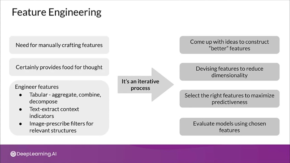
Feature Engineering
Manual Dimensionality Reduction: Case Study with Taxi Fare dataset
CSV_COLUMNS = [
'fare_amount',
'pickup_datetime', 'pickup_longitude', 'pickup_latitude',
'dropoff_longitude', 'dropoff_lattidude',
'passenger_count', 'key'
]
LABEL_COLUMN = 'fare_amount'
STRING_COLS = ['pickup_datetime']
NUMERIC_COLS = ['pickup_longitude', 'pickup_latitude',
'dropoff_longitude', 'dropoff_lattidude',
'passenger_count']
DEFAULTS = [[0.0], ['na'], [0.0], [0.0], [0.0], [0.0], [0.0], ['na']]
DAYS = ['Sun', 'Mon', 'Tue', 'Wed', 'Thu', 'Fri', 'Sat']
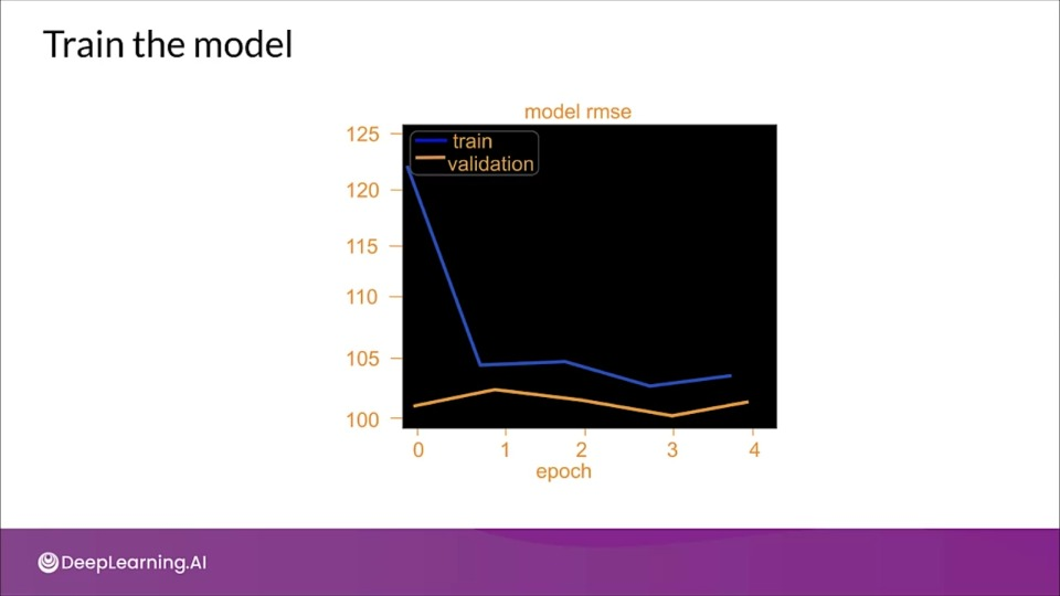
# Build a baseline model using raw features
from tensorflow.leras import layers
from tensorflow.keras.metrics import RootMeanSquared as RMSE
dnn_inputs = layers.DenseFeatures(features_columns.values())(inputs)
h1 = layers.Dense(32, activation='relu', name='h1')(dnn_inputs)
h2 = layers.Dense(8, activation='relu', name='h2')(h1)
output = layers.Dense(1, actiation='linear', name='fare')(h2)
model = keras.models.Model(inputs, output)
model.compile(optimizer='adam', loss='mse',
metrics=[RMSE(name='rmse'), 'mse'])
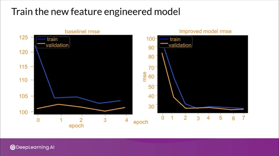
Increasing model performance with Feature Engineering
- Carefully craft features for the data types
- Temporal (pickup date & time)
- Geographical (latitude and longitude)
Handling temporal features
def parse_datetime(s):
  if type(s) is not str:
    s = s.numpy().decode('utf-8')
  return datetime.datetime.strptime(s, "%Y-%m-%d %H:%M:%S %Z")

def get_dayofweek(s):
  ts = parse_datetime(s)
  return DAYS[ts.weekday()]

@tf.function
def dayofweek(ts_in):
  return tf.map_fn(
    lambda s: tf.py_function(get_dayofweek, inp=[s],
              Tout=tf.string),
    ts_in)
Geological features
def euclidean(params):
  lon1, lat1, lon2, lat2 = params
  lodiff = lon2 - lon1
  latdiff = lat2 - lat1
  return tf.sqrt(londiff * longdiff + latdiff * latdif)
Scaling latitude and longitude
def sclae_longitude(lon_column):
  return (lon_column + 78)/8.   # Min: -70 | Max: +78

def scale_latitude(lat_column):
  return (lat_column - 37/8.    # Min:  37 | Max: 45
Preparing the transformations
def transform(inputs, numeric_cols, string_cols, nbuckets):
  ...
  feature_columns = {
    colname: tf.feature_column.numeric_column(colname)
      for colname in numeric_cols
  }

  for lon_col in ['pickup_longitude', 'dropoff_longitude']:
    transformed[lon_col] = layers.Lambda(scale_longitude,
        ...)(inputs[long_col])

  for lat_col in ['pickup_latitude', 'dropoff_latitude']:
    transformed[lat_col] = layers.Lambda(scale_latitude,
        ...)(inputs[lat_col])
Bucketizing and feature crossing
Unless the specific geometry of the earth is relevant to your data, a bucketized version of the map is likely to be more useful than the raw inputs.
def transform(inputs, numeric_cols, string_cols, nbuckets):
  ...
  latbucksts = np.linspace(0, 1, nbuckets).tolist()
  lonbuckets = ...
  b_plat = fc.bucketized_column(
    feature_columns['pickup_latitude'], latbuckets)
  b_dlat = # Bucketize 'dropoff_latitidue'
  b_plon = # Bucketize 'pickup_longitude'
  b_dlon = # Bucketize 'dropoff_longitude'

ploc = fc.cross_column([b_plat, b_plon], nbuckets * nbuckets)
dloc = # Feature corss 'b_dlat' and 'b_dlon'
pd_pair = fc.crossed_column([ploc, dloc], nbuckets ** 4)

Feature_columns['pickup_and_dropoff'] = fc.embedding_column(pd_pair, 100)
Algorithmic Dimensionality Reduction
Linear dimensionality reduction
- Linearly project $n$-dimensional data onto a $k$-dimensional subspace ($k < n$, often $k << n$)
- There are infinitely many $k$-dimensional subspace we can project the data onto
- Which one should we choose?
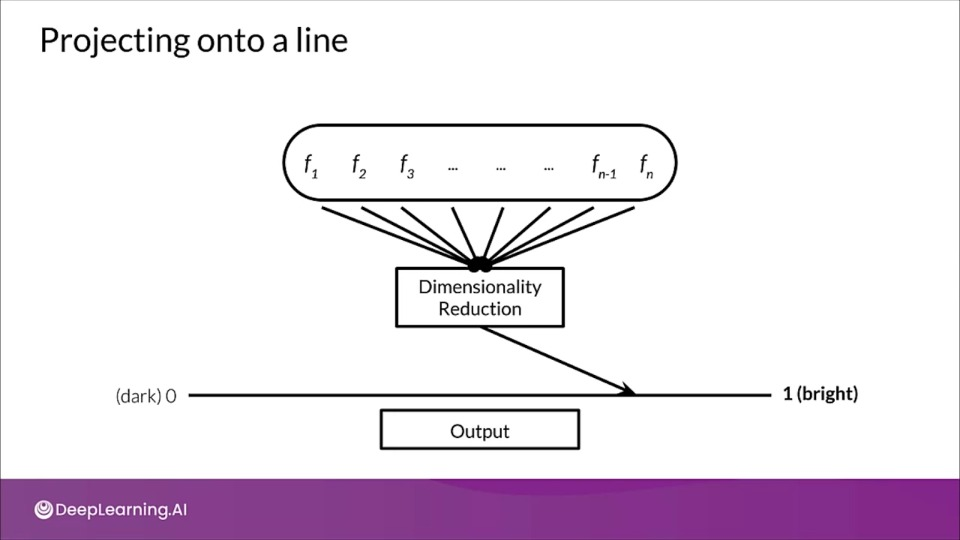
Projecting onto a line
- Let's thing of features as vectors existing in a high-dimensional space.
- Vectors being high dimensional is difficult to visualize, but if we project onto a lower dimension, allows us to visualize the data more easily. This is referred to as embedding.
Best k-dimensional subspace for projection
Classification: maximum separation among classes
Example: Linear Discriminant analysis (LDA)
Regression: maximize correlation between projected data and output variable
Example: Partial Least Squares (PLS)
Unsupervised: retain as much data variance as possible
Example Principal component analysis (PCA)
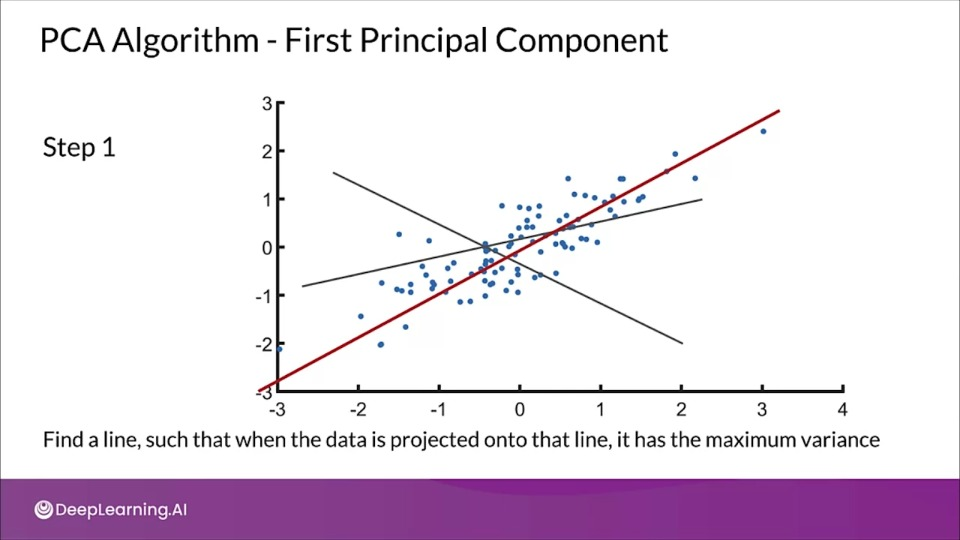
Principal Components Analysis
- Relies on eigen-decomposition (which can only be done for square matrices)
- PCA is a minimization of the orthogonal distance
- Widely used method for unsupervised & linear dimensionality reduction
- Accounts for variance of data in as few dimensions as possible using linear projections
PCA performs dimensionality reduction in two steps:
-
PCA rotates the samples so that they are aligned with the coordinate axis.
PCA also shifts the samples so that they have a mean of zero
Principal components (PCs)
- PCs maximize the variance of projections
- PCs are orthogonal
- Gives the best axis to project
- Goal of PCA: Minimize total squared reconstruction error
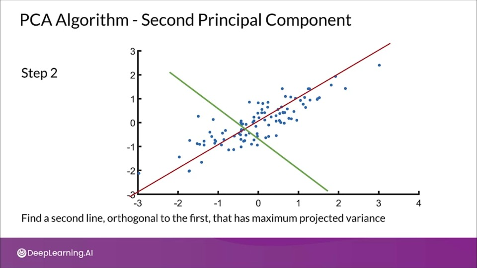
 Repeat until we a have k orthogonal lines
from sklearn.decomposition import PCA

# PCA that will retain 99% of the variance
pca = PCA(n_components=0.99, whiten=True)
pca.fit(X)
X_pca = pca.transform(X)
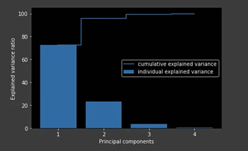
Plot the explained variance
tot = sum(pca.e_vals_)
var_exp = [(i / tot) * 100 for i in sorted (pca.e_evals_, reverse=True)
cum_var_exp = np.cumsum(var_exp)
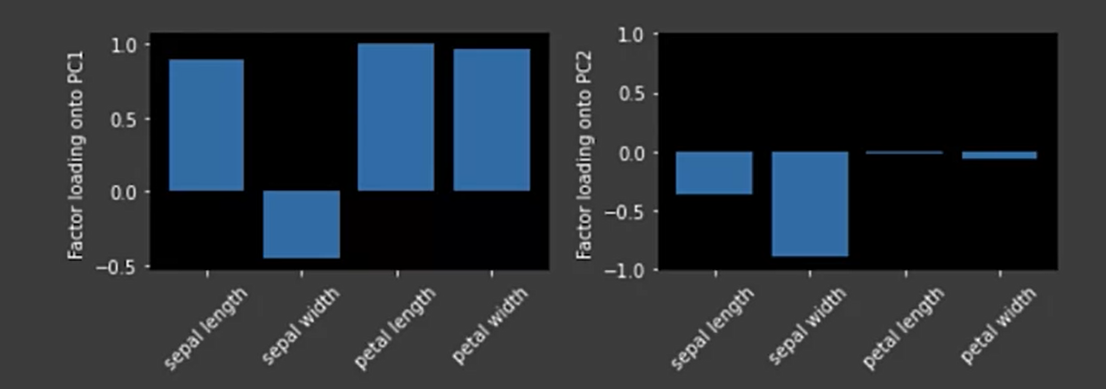
PCA factor loadings
The factor loadings are the unstandardized values of the eigenvectors.
When to use PCA?
Strengths:
- A versatile technique
- Fast and simple
- Offers several variations and extensions (e.g., kernel/sparse PCA)
Weaknesses:
- Result is not interpretable
- Requires setting threshold for cumulative explained variance
Other Techniques
Unsupervised
- Latent Semantic Indexing/ Analysis (LSI and LSA) (SVD)
- Independent Component Analysis (ICA)
Matrix Factorization
- Non-Negative Matrix Factorization (NMF)
Latent Methods
- Latent Dirichlet Allocation (LDA)
Singular Value Decomposition (SVD)
- SVD decomposes non-square matrices
- Useful for sparse matrices and matrices that are not square matrices as produced by TF-IDF.
- Removes Redundant features from the dataset
Independent Component Analysis
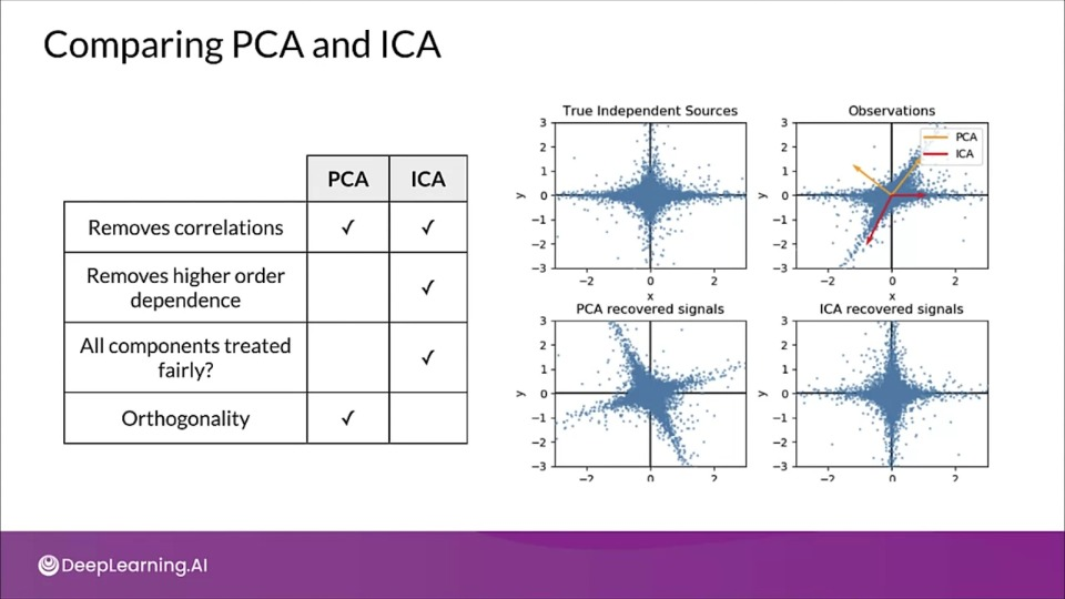
- PCA seeks directions in feature space that minimize reconstructions error, or for uncorrelated factors.
- ICA seeks directions that are most statistically independent
- ICA addresses higher order dependence
How does ICA work?
- Assume there exists independent signals:
- $S = [s_1(t), s_2(t), ..., s_N(t)]$
- Linear combinations of signals: $Y(t) = A S(t)$
- Both $A$ and $S$ are unknown
- $A$ - mixing matrix
- Goal of ICA: recover original signal, $S(t)$ from $Y(t)$
Comparing PCA and ICA
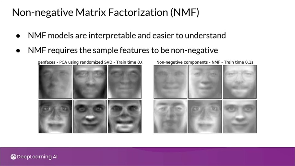
Non-negative Matrix Factorization (NMF)
- NMF model are interpretable and easier to understand
- NMF requires the sample features to be non-negative
- NMF models are interpretable but it can't be applied to all datasets
- It requires the sample features to non-negative.
Dimensionality Reduction Techniques
Dimensionality Reduction Techniques
If you wish to dive more deeply into dimensionality reduction techniques, feel free to check out these optional references. You won’t have to read these to complete this week’s practice quizzes.
Quantization and Pruning — Mobile, IoT, and Similar Use Cases
Factors driving new trend of edge computing
- Demands move ML capability from cloud to on-device
- Cost-effectiveness
- Compliance with privacy regulations
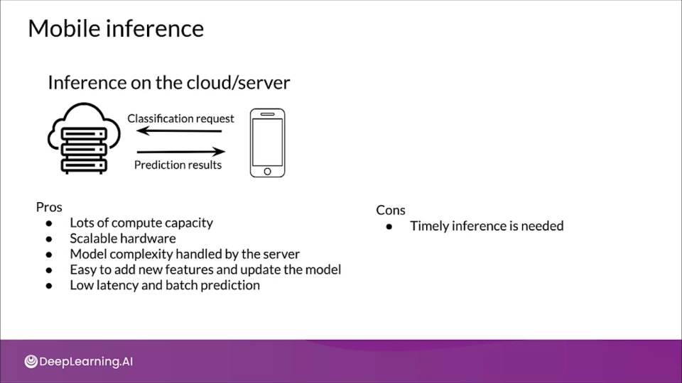
Online ML inference
- To generate real-time predictions you can:
- Host the model on a server
- Embed the model in the device
- Is it faster on a server, or on-device?
- Mobile processing limitations?
Mobile inference
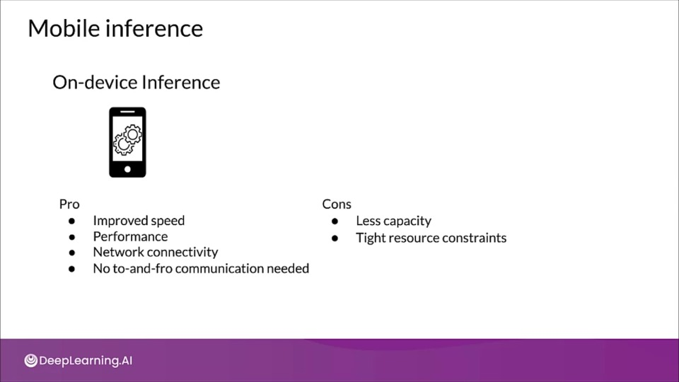
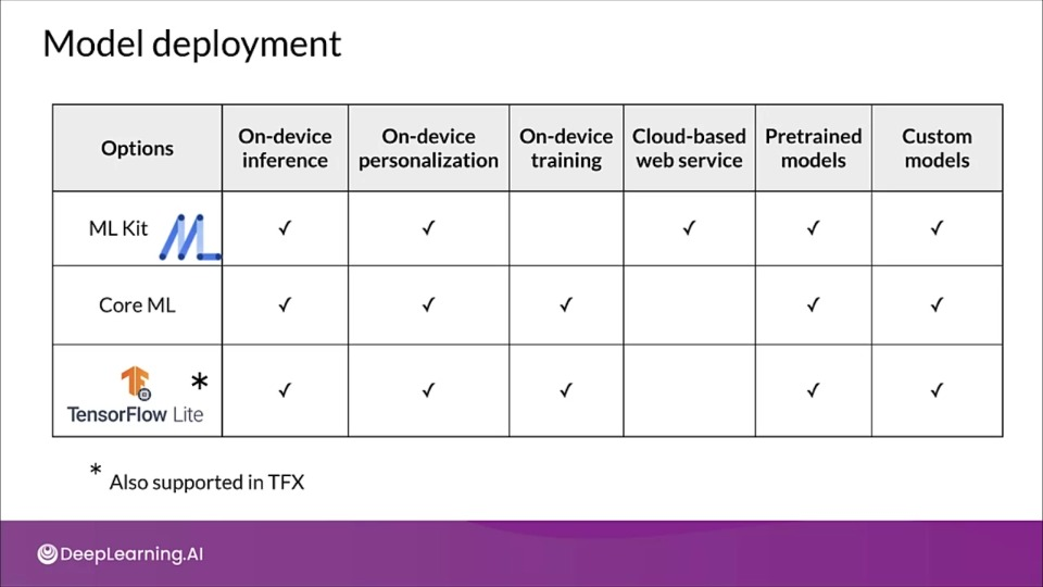
Model development
Benefits and Process of Quantization
Quantization involves transforming a model into an equivalent representation that uses parameters and computations at a lower precision.
This improves model execution performance and efficiency but at the cost of slightly lower model accuracy.

Think of a picture, which is a grid of pixels, each pixel has a certain number of bits. Now if we try reducing the continuous color spectrum of real life to discrete colors, we're quantizing or approximating the image.
Beyond a certain point it may get harder to recognize what the data/image really is.
Why quantize neural netowrks?
- Neural networks have many parameters and take up space
- Shrinking model file size
- Reduce computational resources
- Make models run faster and use less power with low-precision
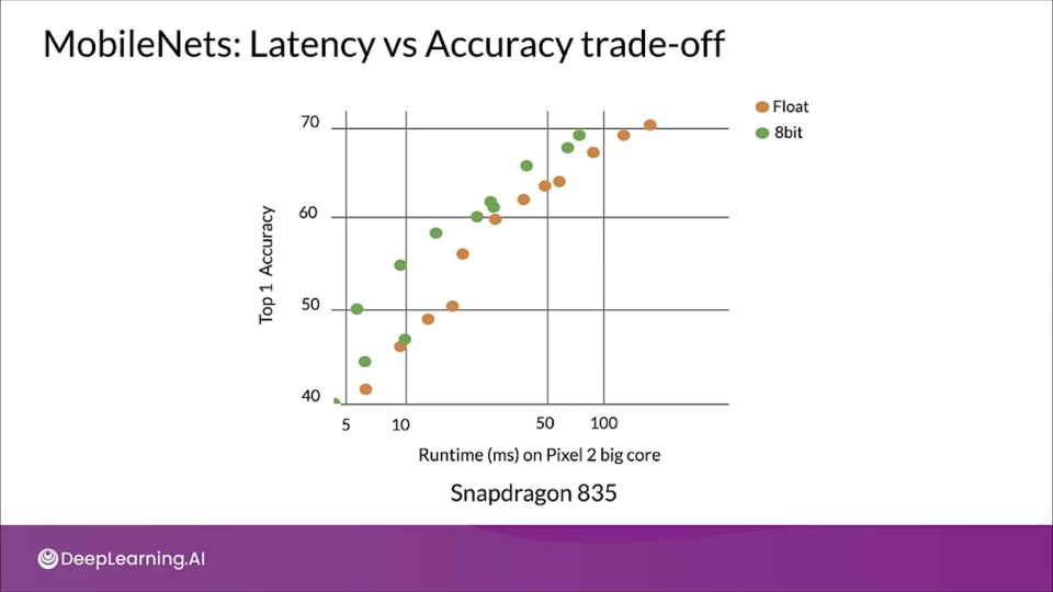
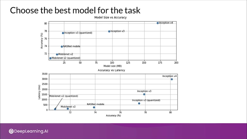
MobileNets: Latency vs Accuracy trade-off
MobileNets are family of small, low-latency, low-power models parameterized to meet the resource constraints of a variety of use cases.
Benefits of quantization
- Faster compute
- Low memory bandwidth
- Low power
- Integer operations supported across CPU/DSP/NPUs
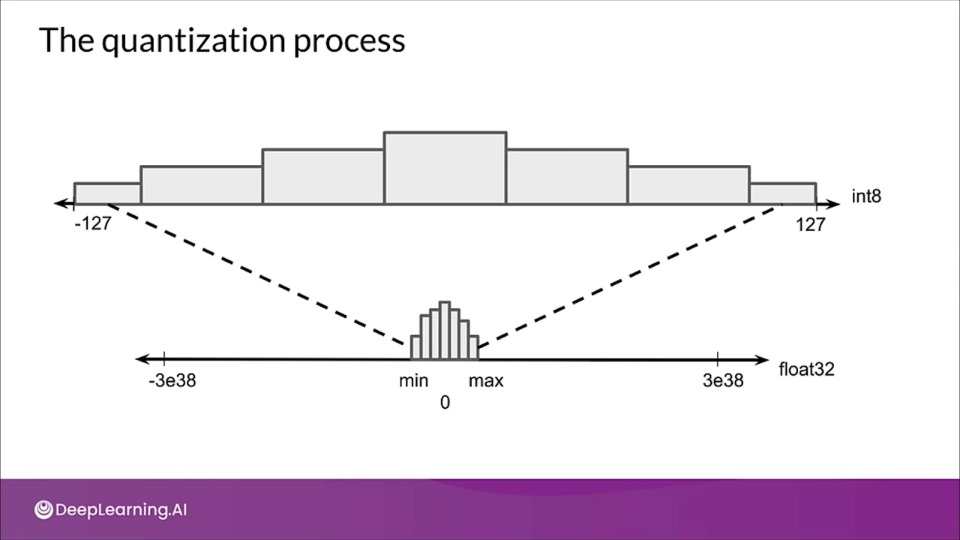
The quantization process
The weights and activations for a particular layer often tend to lie in a small range, which can be estimated beforehand. That's why we don't need to store the range in the same data type. Therefore we can concentrate the fewer bits within a smaller range.
Find the maximum absolute weight value, $m$, then maps the floating point range $-m$ to $+m$ to the fixed-point range $-127$ to $+127$.
What parts of the mode are affected?
- Static parameters (like weights of the layers)
- Dynamix parameters (like activations inside networks)
- Computation (transformations)
Trade-offs
- Optimizations impact model accuracy
- Difficult to predict ahead of time
- In rare cases, models may actually gain some accuracy
- Undefined effects on ML interpretability.
Choose the best model for the task
Post Training Quantization
In this technique an already trained TensorFlow model size is reduced by using TensorFlow Lite converter to save into TensorFlow Lite format.
- Reduced precision representation
- Incur small loss in model accuracy
- Joint optimization for mode and latency
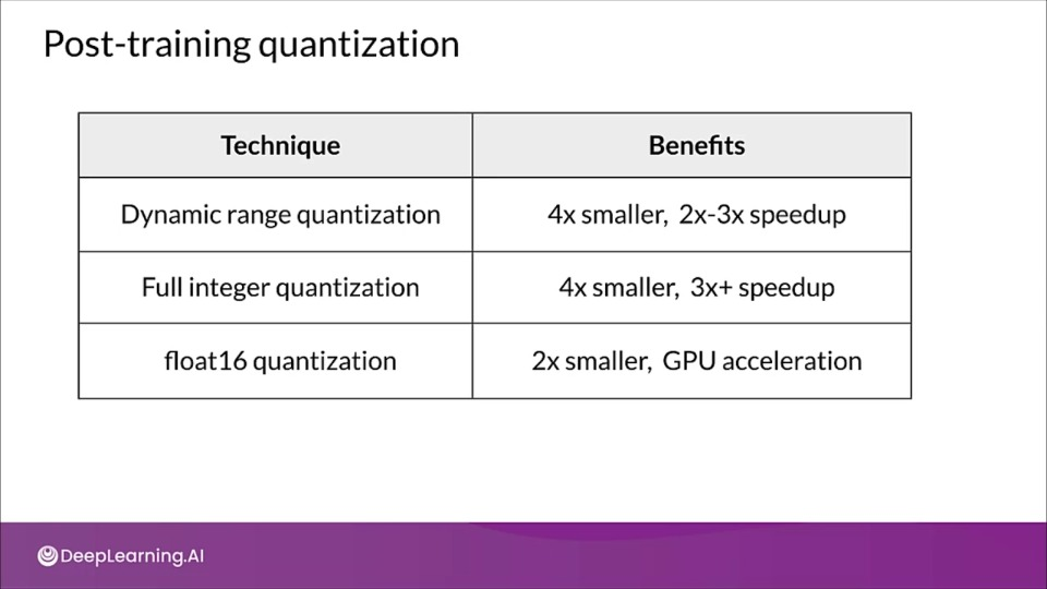
- In dynamic range quantization, during inference the weights are converted back from eight bits to floating point and activations are computed using floating point kernels.
- This conversion is done once, cached to reduce latency
import tensorflow as tf

converter = tf.lite.TFLiteConverter.from_saved_model(saved_model_dir)
coverter.optimizations = [tf.lite.Optimize.OPTIMIZE_FOR_SIZE]

tflite_quant_model = converter.convert()
Model accuracy
- Small accuracy loss incurred (mostly for smaller network)
- Use the benchmarking tools to evaluate model accuracy
- If the loss of accuracy drop is not within acceptable limits, consider using quantization-aware training
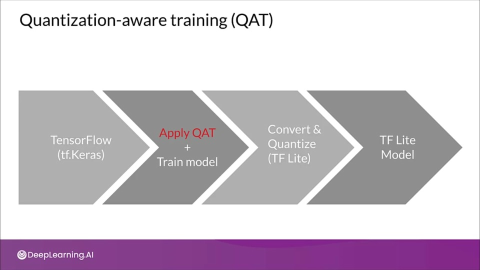
Quantization Aware Training
Quantization aware training adds fake quantization operations to the mode so it can learn to ignore the quantization noise during training.
- Inserts fake quantization (FQ) nodes in the forward pass
- Rewrites the graph to emulate quantized inference
- Reduces the loss of accuracy due to quantization
- Resulting model contains all data to be quantized according to spec
QAT on entire model
import tensorflow_model_optimization as tfmot

model = tf.keras.Sequential([
    ...
])

# Qunatize the entire model.
quntized_model = tfmot.quantization.keras.quantize_model(model)

# Continue with training as usual
quantized_model.compile(...)
quantized_model.fit(...)
Quantize parts(s) of a model
import tensorflow_model_optimization as tfmot
quanitze_annotate_layer = tfmot.quanitzation.keras.quanitze_annotate_kayer

model = tf.keras.Sequential([
    ....
    # Only anotated layers will be quantized
    quantize_annotate_layer(Conv2D()),
    quantize_annotate_layer(ReLU()),
    Dense(),
    ...
])

# Quantize the model
quantized_model = tfmot.quantization.keras.quantize_apply(model)
Quantize custom Keras layer
quantize_annotate_layer = tfmot.quantization.keras.quantize_annotate_layer
quantize_annotate_model = tfmot.quantization.leras.quantize_annotate_model
quantize_scope = tfmot.quatization.keras.quantize_scope

model = quantize_annotate_model(tf.keras.Sequential([
    quantize_annotate_layer(CustomLayer(20, input_shape=(20,)),
                                                    DefaultDenseQuantizeConfig()),
    tf.keras.layers.Flatten()
]))

# `quantize_apply` requires mentioning `DefaultDenseQuantizeConfig` with
# `quantize_scope`
with quantize_scope(
    {'DefaultDenseQuantizeConfig': DefaultDenseQuantizeConfig,
     'CustomLayer': CustomLayer}):
    # Use 'quantize_apply` to actually make the model quantization aware
    quant_aware_model = tfmot.quantization.keras.quantize_apply(model)
Quantization
Quantization
If you wish to dive more deeply into quantization, feel free to check out these optional references. You won’t have to read these to complete this week’s practice quizzes.
Pruning
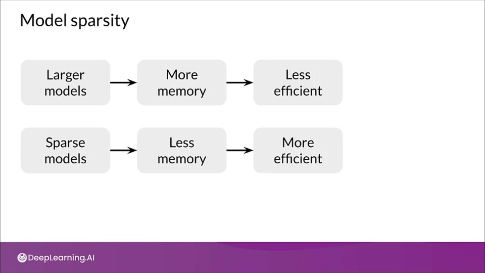
Pruning increases the efficiency of model by removing parts (connections) of model that do not contribute to substantially to producing accurate results.
Model Sparsity
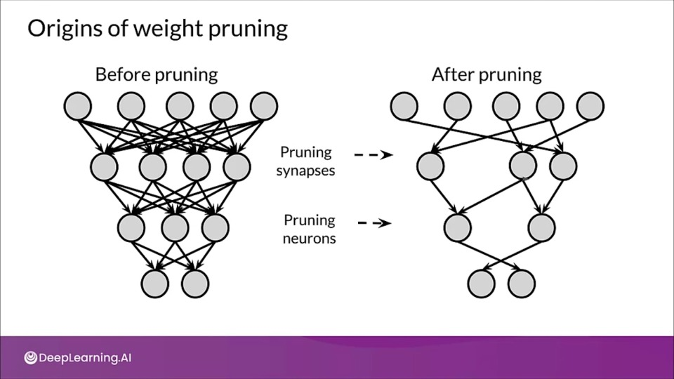
Origins of weight pruning
The first major paper advocating sparsity and neural networks dates back from 1990, in "Optimal of Brain Damage" written by Yann LeCun, John S.Denker, and Sara A. Solla.
At that time post pruning NN was already a trendy choice to reduce the size of models. runing was mainly done by using magnitude as an approximation for saliency to determine less useful connections.
- Intuition being smaller the weight smaller the effect was on the output.
- The saliency of each weight was estimated, defined by change in the loss function upon applying a perturbation to the nodes in the network. Finally retraining the model again.
- But retraining became a lot harder.
- The answer came with "lottery ticket hypothesis"
Lottery ticket Hypothesis
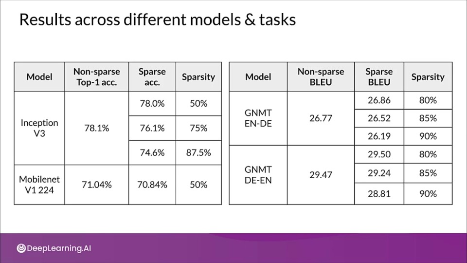
As the network size increases, the number of possible subnetworks and the probability of finding the ‘lucky subnetwork’ also increase. As per the lottery ticket hypothesis, if we find this lucky subnetwork, we can train small and sparsified networks to give higher performance even when 90 percent of the full network’s parameters are removed.
Finding Sparse Neural Networks
"A randomly-initialized, dense neural network contains a subnetwork that is initialized such that — when trained in isolation — it can match the test accuracy of the original network after training for at most the same number of iterations" - Jonathan Frankle and Michael Carbin
Basically instead of fine-tuning weights, just reset the weight to original value and retain.
This lead to the acceptance of the idea that over parameterized dense networks containing several sparse subnetworks with varying performances, and one of these subnetworks is the winning ticket, which perform all others.
Pruning research is evolving
- The new method didn't perform well at large sacle
- The new method failed to identify the randomly initialized winners
- Active area of research
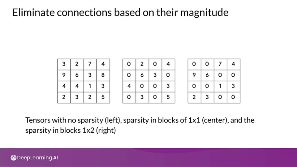
Eliminate connections based on their magnitude
TensorFlow includes a weight pruning API, which can iteratively remove connections based on their magnitude during training.
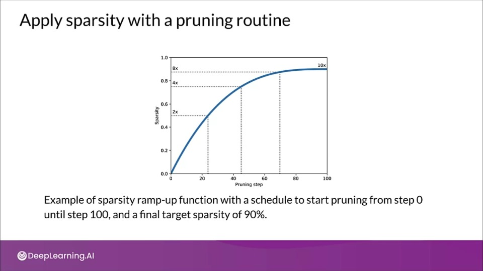
Sparsity increases with training
 tion="Image source: TensorFlow Model Optimization Toolkit — Pruning API (morioh.com) Black cells indicate where the non-zero weights exist as pruning is applied to a tensor." >}}
What's special about pruning?
- Better storage and/or transmission
- Gain speedups in CPU and some ML accelerators
- Can be used in tandem with quantization to get additional benefits
- Unlock performance improvements
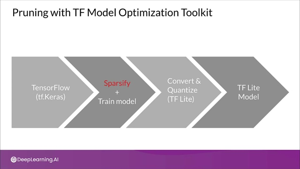
Pruning with TF Model Optimization Toolkit iwth Keras
import tensorflow_model_optimization as tfmot

model = build_your_model()
pruning_schedule = tfmot.sparsity.keras.PolynomialDecay(
                                            initial_sparsity=0.5, final_sparsity=0.8,
                                            begin_Step=2000, end_step=4000)

model_for_pruning = tfmot.sparsity.keras.prune_low_magnitude(
                                            model,
                                            pruning_scehdule=pruning_schedule)

...
model_for_pruning.fit()
Pruning
Pruning
If you wish to dive more deeply into pruning, feel free to check out these optional references. You won’t have to read these to complete this week’s practice quizzes.