Week 3 — High Performance Modeling"

Knowledge Distillation, Data Parallelism, ETL Process

Distributed Training

Rise in coputational requirements

• At first, training models is quick and easy
• Training models becomes more time-consuming
  • With more data
  • With larger models
• Longer training → More epochs → Less efficient
• Use distributed training approaches

Types of distrubued training

• Data parallelism: In data parallelism, models are replicated onto different accelerators (GPU/TPU) and data is split between them.
  • Model agnostic i.e., can be applied to any neural architecture
• Model parallelism: When models are too large to fit on a singe device then they can be divided into partitions, assigning different partitions to different accelerators.

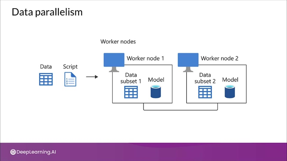
Data parallelism

The model is copied to workers, and data is split between them. That means workers should have enough memory to store the model and perform the forward and backward pass. After backprop the changes are shared among the workers and weights are updated.

Distributed training using data parallelism

1. Synchronous training
   • All workers train and complete updated in sync
   • Supported via all-reduce architecture
2. Asynchronous training
   • Each worker trains and completes updates separately
   • Supported via parameter server architecture
   • More efficient, but can result in lower accuracy and slower convergence.

Making your model distribute-aware

• If you want to distribute a model:
  • Supported in high-level APIs such as Keras/Esstimators
  • For more control, you can use custom training loops

tf.distribute.Strategy

• Library in TensorFlow for running a computation in multiple devices
• Supports distribution strategies for high-level APIs like Keras and custom training loops
• Convenient to use with little or no code changes.

Distribution Strategies supported by tf.distribute.Strategy

• One Device Strategy
• Mirrored Strategy
• Parameter Server Strategy
• Multi-Worker Mirrored Strategy
• Central Storage Strategy
• TPU Strategy

One Device Strategy

• Single device - no distribution
• Typical usage of this strategy is testing your code before switching to other strategies that actually distribute your code.

Mirrored Strategy

This strategy is typically used on one machine with multiple GPUs.

• Supported synchronous distributed training.
• Creates a replica per GPU <> Variables are mirrored
• Weight updating is done using efficient cross-device communication algorithms (all-reduce algorithms)

Fault tolerance

• If a worker gets interrupted, the whole cluster will pause, wait for interrupted worker to restart and then other worker will also restart. After that then can resume from their former state

Parameter Server Strategy

• Some machines are designed as workers and others as parameter servers.
  • Parameter servers store variables so that workers can perform computations on them.
• Implements asynchronous data parallelism by default.

Fault tolerance

• Catastrophic failures in one worker would cause failure of distribution strategies.
• How to enable fault tolerance in case a worker dies?
  • By restoring training state upon restart from job failure.
  • Keras implementation: BackupAndRestore callback.

High Performance Ingestion

Why input pipelines?

Data at times can't fit into memory and sometimes, CPUs are under-utilized in compute intensive tasks like training a complex model.

You should avoid these inefficiencies so that you can make the most of the hardware available $\rightarrow$ Use input pipelines.

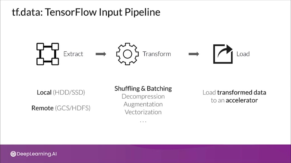
tf.data: TensorFlow Input Pipeline

An improved ETL process

Overlap different parts of ETL by using a technique known as software pipelining.

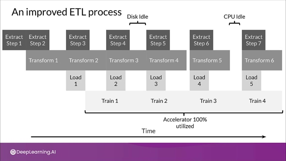
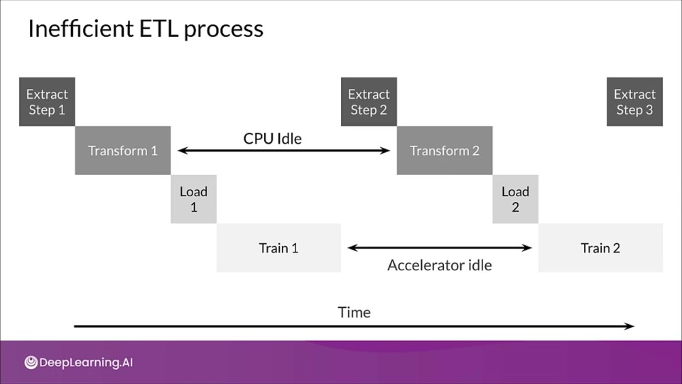
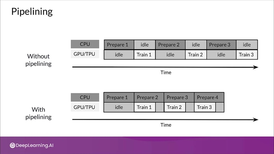
Pipelining

Through pipelining we can overcome CPU bottlenecks by overlapping CPU pre-processing and model execution by accelerators.

With pipeline while GPU is training, the CPU starts preparing data for next training step, thus decreasing the idle time.

How to optimize pipeline performance?

• Prefetching
• Parallelize data extraction and transformation
• Caching
• Reduce Memory

Optimize with prefetching

Overlap the work of a producer with a work of a consumer.

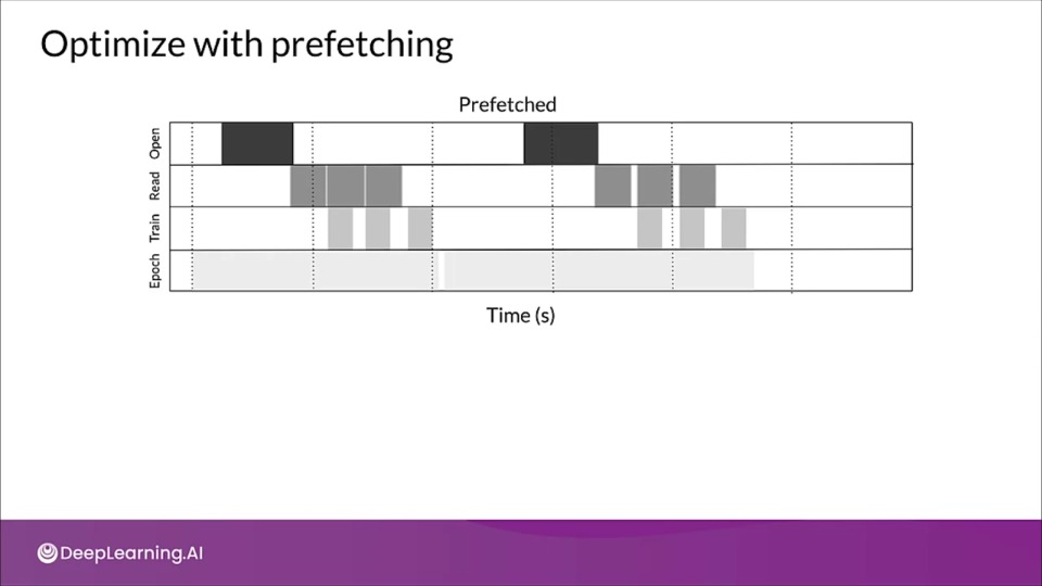
This transformation uses a background thread and an internal buffer to prefetch elements from the input dataset ahead of time before they are requested.

benchmark(
    ArtificialDataset()
    .prefetch(tf.data.experimental.AUTOTUNE)
)

Ideally the number of elements to prefetch should be equal to or greater than the number of batches consumed by a single training step.

We can manually tune this value, or set it to tf.data.experimental.AUTOTUNE

Parallelize data extraction

A pipeline that run locally might become bottleneck when the data is stored remotely like in cloud or in HDFS due to:

• Time-to-first-byte: Prefer local storage as it takes significantly longer to read data from remote storage.
• Read throughput: Maximize the aggregate bandwidth of remote storage by reading more files instead of single one.

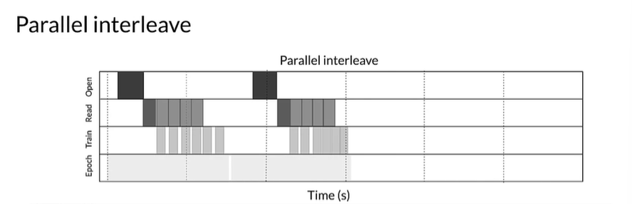
Parallelize the data loading step including interleaving contents of other datasets.

benchmark(
    tf.data.Dataset.range(2)
    .interleave(
        ArtificialDataset,
        num_parallel_calls=tf.data.experimental.AUTOTUNE # Level of parallelis
    )
)

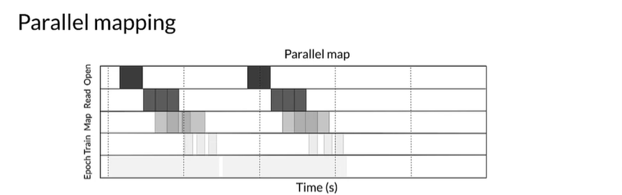
Parallelize data transformation

Often times, the input elements may need to be preprocessed.

• Post data loading, the inputs may need preprocessing
• Element-wise preprocessing can be parallelized across CPU cores
• The optimal value for the level of parallelism depends on:
  • Size and shape of training data
  • Cost of the mapping transformation
  • Load the PCU is experiencing currently
• With tf.data you can use AUTOTUNE to set parallelism automatically

benchmark(
    ArtificialDataset()
    .map(
        mapped_function,
        num_paralllel_calls=tf.data.AUTOTUNE
    )
)

Improve training time with caching

• In-memory: tf.data.Dataset.cache()
• Dish: tf.data.Dataset.cache(filename=...)

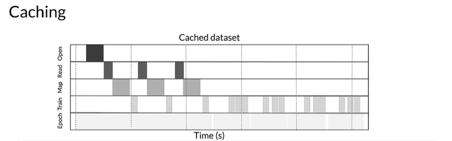
If user defined mapping transformation function is expensive it makes sense to cache the dataset as long as it fits in memory.

If the user-defined function increases the space required to store the dataset beyond the cache capacity either applied it after cache transformation or consider pre-processing the data before your training job to reduce the resource requirement.

benchmark(
    ArtificialDatset().map(mapped_function).cache(), 5
)

Training Large Models - The Rise of Giant Neural Nets and Parallelism

Rise of giant neural networks

• In 2014, the ImageNet winner was GoogleNet with 4 million parameters and scoring a 74.8% top-1 accuracy.
• In 2017, Squeeze-and-excitation networks achieved 82.7% top-1 accuracy with 145.8 million parameters.

36 fold increase in the number of parameters in just 3 years!

Issues with training larger networks

• GPU memory only increased by factor ~3
• Saturated the amount of memory available in Cloud TPUs
• Need for large-scale training of giant neural networks

Overcoming memory constraints

1. Strategy #1 - Gradient Accumulation

   • Split batches into mini-batches and only perform backprop after whole batch.

   During backprop, the model isn't updated with each mini-batch, and instead, the gradients are accumulated. When the batch completes, all the accumulated gradients of the mini-batches are used for the backprop to update the model.

2. Strategy #2 - Memory swap

   • Copy activations between CPU and memory, back and forth.

   Since there isn't enough storage on the accelerator, you copy activations back to memory and then back to the accelerator. But this is slow.

Parallelism revisited

Data parallelism: In data parallelism, models are replicated onto different accelerators (GPU/TPU) and data is split between them.

Model parallelism: When models are too large to fit on a single device then they can be divided into partitions, assigning different partitions to different accelerators.

Sophisticated methods for model parallelism make sure that each worker is similarly busy by analyzing the computational complexity of each layer.

This enables training of larger networks but suffers from a large hit in performance since workers are constantly waiting for each other and only one can perform updates at a given time.

Challenges in data parallelism

Two factors contribute to the communication overhead across all models:

1. An increase in data parallel workers
2. An increase in GPU compute capacity

The frequency of parameter synchronization affects both statistical and hardware efficiency:

• Synchronizing at the end of every mini-batch reduces the staleness of weights used to compute gradients ensuring good statistical efficeincy.

  But this requires each GPUs to wait for gradients from other GPUs, i.e., impacting hardware efficiency.

Communication stalls also become inevitable in data parallelism making the communication can often dominate total execution time.

Challenges keeping accelerators busy

• Accelerators have limited memory
• Model parallelism: large networks can be trained
  • But, accelerator compute capacity is underutilized (Other accelerators might have to wait until previous one finishes)
• Data parallelism: train same model with different input data
  • But, the maximum model size an accelrator can support is limited.

Pipeline parallelism using GPipe

In this diagram, F refers to the forward pass while B refers to the backward pass distributed among the accelerators

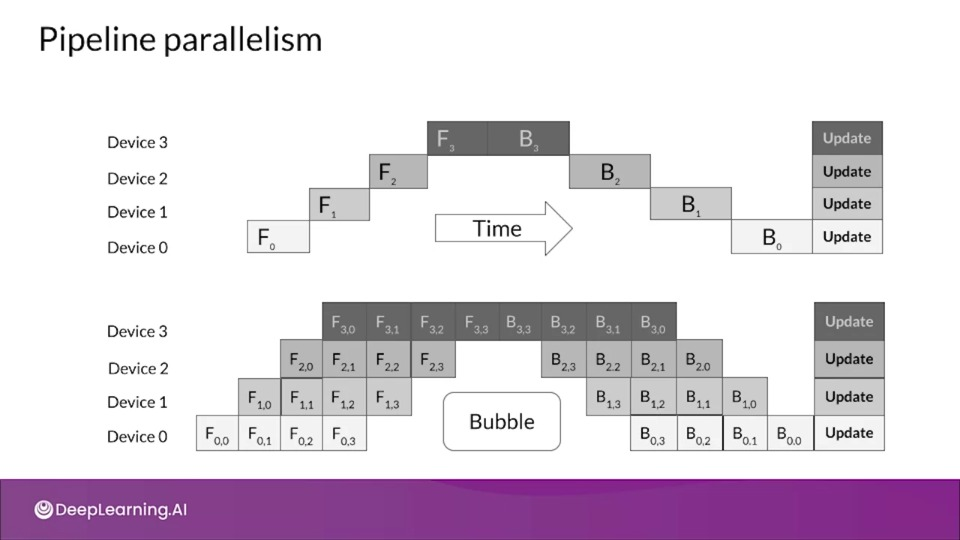
Google's GPipe is an open source library for efficiently training large-scale models using pipeline parallelism.

In the diagram at the bottom, the GPipe divides the input mini-batch into smaller micro-batches, enabling different accelerators to work on separate micro-batches at the same time.

It inserts communication primitives at the partition boundaries

Automatic parallelism to reduce consumption

Synchronous stochastic Gradient accumulation across micro-batches, sot that model quality is preserved.

• Integrates both data and model parallelism
  • Divide mini-batch data into micro-batches
  • Different workers work on different micro-batches in parallel
  • Allow ML models to have significantly more parameters

High-Performance Modeling

If you wish to dive more deeply into high-performance modeling, feel free to check out these optional references. You won’t have to read these to complete this week’s practice quizzes.

• Distributed training
• Data parallelism
• Pipeline parallelism
• GPipe

Teacher and Student Networks

We can also try to capture or distill the knowledge that has been learned by a model in a more compact model by a style of learning known as Knowledge Distillation.

Sophisticated models and their problems

• Larger sophisticated models become complex
• Complex models learn complex tasks
• Can we express this learning more efficiently?

Is it possible to 'distill' or concentrate this complexity into smaller networks?

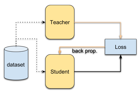
Knowledge distillation

Knowledge distillation is a way to train a small model to mimic a larger model or even ensemble of models by first training a complex model achieving a high level of accuracy and then using that model as teacher model for a simpler student model.

• Duplicate the performance of a complex model in a simpler model
• Idea: Create a simple 'student' model that learns from a complex 'teacher' model

Source: [Giang Nguyen](https://github.com/giangnguyen2412/paper-review-continual-learning/blob/master/distillation.md

Knowledge Distillation Techniques

Teacher and student

• Training objectives of the models vary
• Teacher (normal training)
  • maximises the actual metric
• Student (knowledge transfer)
  • matches p-distribution of the teacher's predictions to form 'soft targets' (The probability of the predictions)
  • 'Soft targets' tell us about the knowledge learned by the teacher

Transferring "dark knowledge" to the student

The way knowledge distillation works is that you transfer knowledge form the teacher to the student by minimizing the loss function in which the target is the distribution of class probabilities predicted by the teacher model

The teacher model's logits from the input to the final softmax layer

• Improve softness of the teacher's distribution with 'softmax temperature' ($T$)
• By raising the temperature in the objective functions of the student and teacher, we can improve the softness of the teacher's distribution

As $T$ grows, you get more insight about which classes the teacher finds similar to the predicted one.

As $T$ decreases, the soft target defined by the teacher network become less informative.

As $T$ =1, It's a normal softmax function.

$$ p_i = \frac{\exp(\frac{z_i}{T})}{\sum_j\exp(\frac{z_j}{T})} $$

The probability $p$ of class $i$ is calculated from the logits $z$ as shown. The $T$ refers to the temperature parameter.

• When T is 1, it acts like standard softmax function

• As $T$ starts growing the probability distribution generated by the softmax function becomes softer, providing more information as to which classes the teacher found more similar to the predicted class.

  Authors of the paper referred it to as "dark knowledge" embedded in the teacher model.

Techniques

Various techniques can be employed to train students to match the teacher's soft targets.

• Approach #1: Weight objectives (student and teacher) and combine during backprop

  Train using both teacher's logits and training labels using normal objective functions, the two objective functions are weighted and combined in backpropagatation.

• Approach #2: Compare distributions of the predictions (Student and teacher) using KL divergence.

  The distributions of the teacher's predictions and teacher's predictions are compared using metric such as KL divergence.

KL divergence

$$ L = (1-\alpha ) L_H + \alpha L_{KL} $$

The Kullback-Leibler divergence here is a metric of the difference between two probability distributions.

Generally knowledge is done by blending two loss functions, choosing a value for $\alpha$ between zero and one and we want the probability distributions of predictions of teacher and student model to be close as possible.

Here :

• $L$ is the cross-entropy loss from the hard labels
• $L_{KL}$ is the Kullabck-Leibler divergence loss from the divergence logits of teacher

How knowledge transfer takes place

When computing the "standard" loss between student's prdicted class probabilities and the ground truth "hard" labels, we use a value of the softmax temperature $T$ equal to 1.

In case of heavy data augmentations after training the teacher network, the alpha hyperparmeter should be high in the student network loss function otherwise low alpha parameter would increase the influence of the hard labels that went through aggressive perturbations due to data augmentation.

Case Study - How to Distill Knowledge for a Q&A Task

Traditional model compression suffer from information loss leading to inferior models. To tackle this researchers at Microsoft proposed a two stage multi teacher knowledge distillation method (TMKD) for a web question answering system.

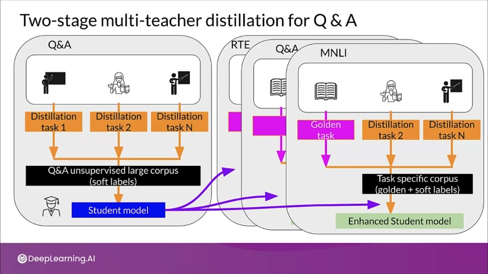
• They first developed a general Q&A distillation task for student model pretraining (right side of diagram), and further fine tune this pre trained student model with a multi-teacher knowledge distillation model (left side of diagram).
• Although the process can effectively reduce the number of parameters and time inference, due to the information loss during knowledge distillation, the performance of the student model is sometimes not on par with that of the teacher.
• This lead of different approach called M on M or many on many ensemble model. Combining both ensemble and knowledge distillation.
• This involves first training multiple teacher models. Then a student model for each teacher model is then trained. Finally, the student models trained from different teachers are ensembled to create the final result.

Make EfficientNets robust to noise with distillation

Carnegie Mellon University trained models with a semi supervised learning method called noisy student:

• In this approach, the knowledge distillation process is iterative.
• The student is purposely kept larger in terms of the number of parameters than the teacher, this enables the model to attain robustness to noisy labels as opposed to traditional knowledge distillation approach.

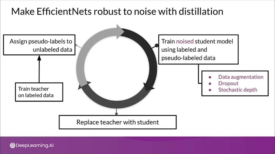
The noising is what pushes the student model to learn harder from pseudo labels.

The teacher model is not noised during the generation of pseudo labels to ensure it's accuracy isn't altered in any way.

Knowledge Distillation

Knowledge Distillation

If you wish to dive more deeply into knowledge distillation, feel free to check out these optional references. You won’t have to read these to complete this week’s practice quizzes.

• Knowledge distillation
• Q&A case study