Week 3 — One hidden layer Neural Networks
May 4, 2021
Shallow Neural Network
Neural Networks Overview
For new notation
We'll use superscript square bracket one to refer to quantities associated with a particular layer.
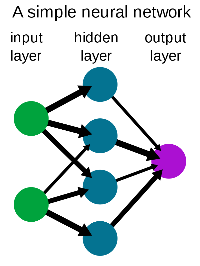
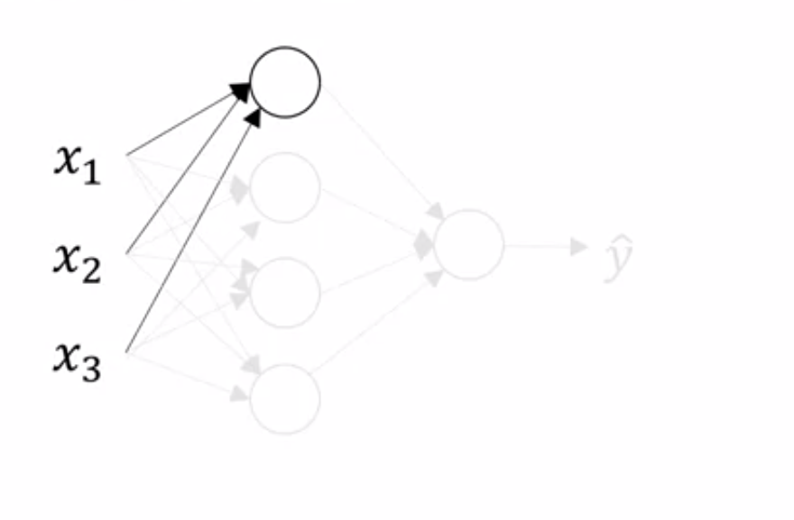
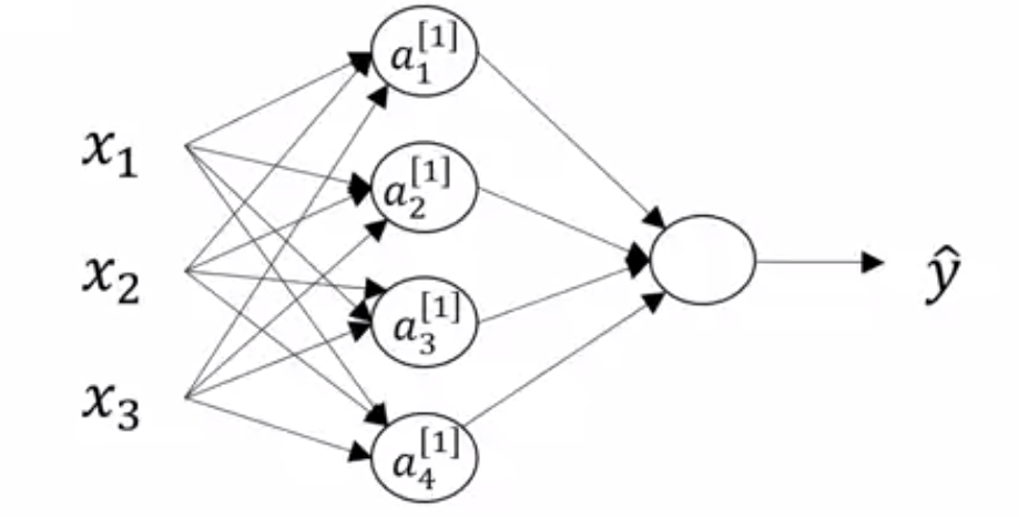
Neural Network Representation
The term hidden layer refers to the fact that in the training set, for these nodes in the middle (the hidden layer neurons) are not observed.
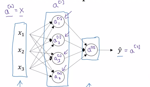
The term $a$ also stands for the activations, we will use it for denoting the outputs/activations of a layer that the layer is passing on to the subsequent layers.
-
Input layer is passing activations $a^{[0]}$ to the hidden layer (which we previously denoting by $X$.
-
The hidden layer will in turn generate its own activations $a^{[1]}$
-
Which is a four dimensional vector b/c the hidden layer has four neurons
- The output layer generates some value $a^{[2]}$ which is just a real number $\hat{y}$.
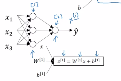
- The parameter associated with the layers will also be denoted with Superscript notations like $W^{[1]}$, $b^{[1]}$. Here,
- $W^{[1]}$ will be $(4. 3)$ dimensional vector for $(\text{noOfNeuronsInCurrentLayer},\text{ noOfNeuronsInPreviviousLayer})$ with each value associated with the connection weights.
- $b^{[1]}$ will be $(4, 1)$ dimensional vector, only stores biases for number of neurons in current layer.
Computing a Neural Network's Output
Let's go a little deeper:
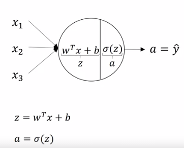
- The first neuron of the hidden layer we just saw earlier gets all inputs from input layer (and so does other neurons in hidden layer)
- It computes
where,
 - The second neuron computes,
- and so does other neurons in the layer.
Once again writing all equations:
$$ z^{[1]}_1 = w^{[1]}_1 X + b_1^{[1]}, \qquad a^{[1]}_1 = \sigma(z^{[1]}_1)\tag{1} $$
$$ z^{[1]}_2 = w^{[1]}_2 X + b_2^{[1]}, \qquad a^{[1]}_2 = \sigma(z^{[1]}_2) \tag{2} $$
$$ z^{[1]}_3 = w^{[1]}_3 X + b_3^{[1]}, \qquad a^{[1]}_3 = \sigma(z^{[1]}_3) \tag{3} $$
$$ z^{[1]}_4 = w^{[1]}_4 X + b_4^{[1]}, \qquad a^{[1]}_4 = \sigma(z^{[1]}_4) \tag{4} $$
To vectorize we can do like this:
Give input $X = a^{[0]}$, then
$z^{[1]} = W^{[1]}a^{[0]} + b^{[1]}$
$a^{[1]} = \sigma(z^{[1]})$
$z^{[1]} = W^{[2]}a^{[1]} + b ^{[2]}$
$a^{[2]} = \sigma(z^{[2]})$
Where $W^{[2]}$ is $(1, 4)$ and $a^{[1]}$ is $(4, 1)$ dimensional matrices.
Vectorizing across multiple examples
If we have defined a neural network like this:
for i=1 to m:
then for $m$ training examples we need,
we can vectorize over m training examples as:
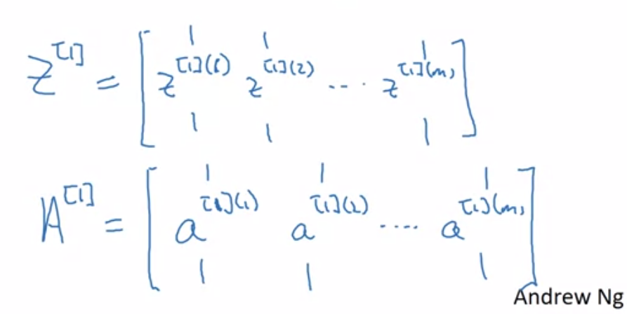
A good thing about these matrices $(Z, A)$ is that they represent vertically hidden units and horizontally they represent training examples.
- That means first row first column represent output from first hidden unit for first training example. The second in the first row output of same first hidden unit for second training example.
- Vertically you get output from second, third and so on hidden unit for the training examples.
Explanation for Vectorized Implementation
Activation Functions
In real world NN, instead of using $\sigma$ (sigmoid) activation function for every problem, we can use other activation functions. So in general we replace $\sigma(z^{[\mathbb{R}]})$ with $g(z^{[\mathbb{R}]})$
The problem with $\tanh$ $\big(tanh(z) = 2\sigma(2z) -1\big)$ or $\sigma$ (sigmoid) function is that when inputs become large, the function saturates at -1 or 1/ 0 or 1 respectively, with derivative extremely close to zero. Thus for backpropagation there is no gradients to work with.
One of the very commonly used Activation function is
Rectified Linear Unit (ReLU)
$$ ReLU(z) = \max(0, z) $$
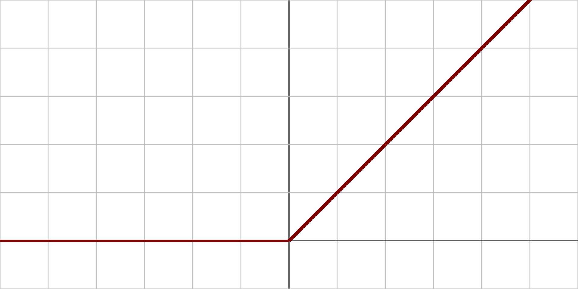
This function is continuous but unfortunately not differentiable at $z=0$ as slope changes abruptly and its derivative is zero for $z<0$. But is practice, it works really well.
But might suffer from dying ReLUs, i.e., that is some neurons stop outputting anything other than 0. In that case Leaky ReLUs and its variant but be better choice.
Leaky ReLU
$$ \text{Leaky ReLU}_\alpha(z) = \max(\alpha z. z) $$
$\alpha$ defines the slope of the function for $z<0$, that is how much it should "leak.
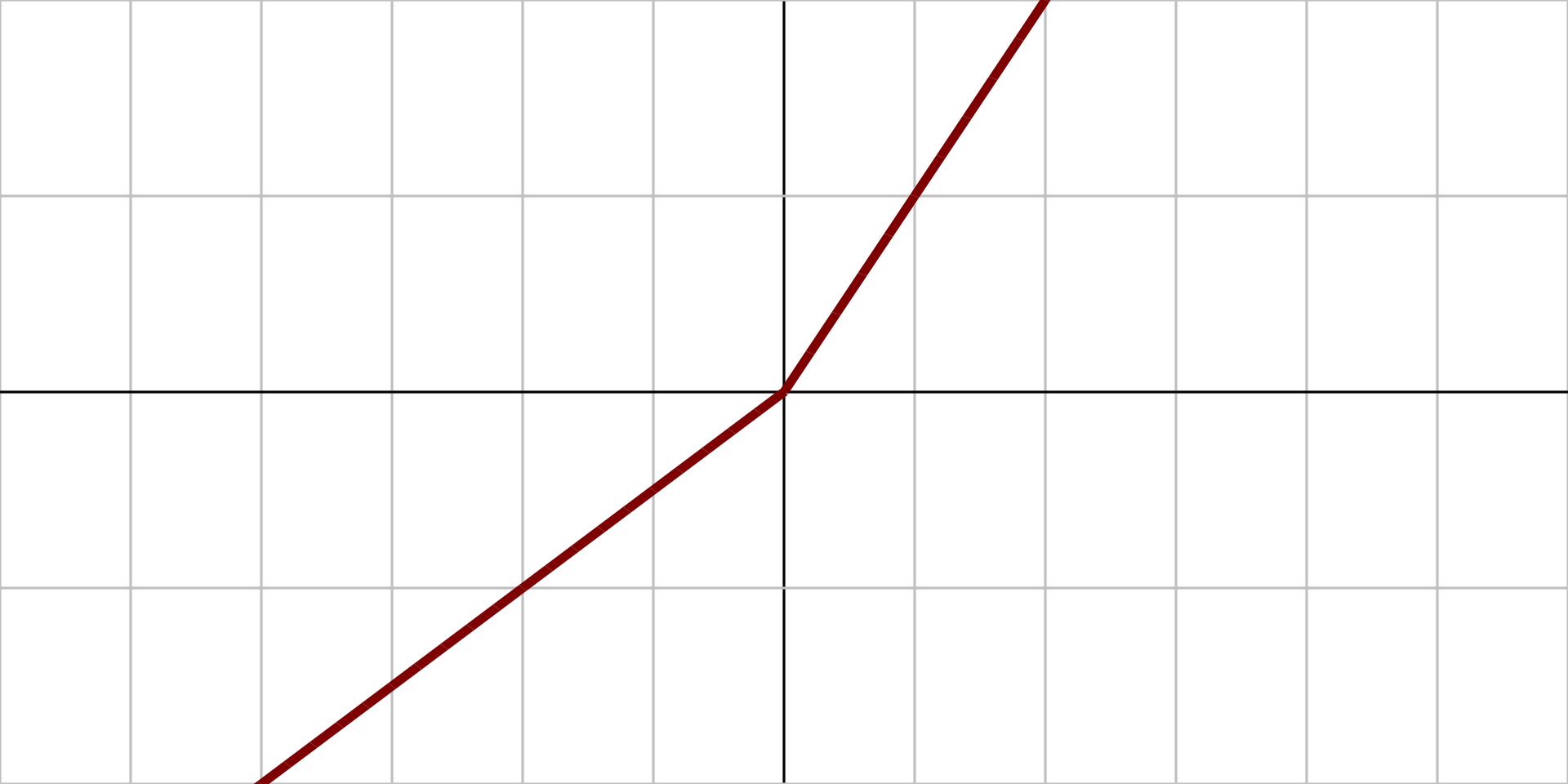
This small slope ensures that the neurons never really "die".
Why do you need non-linear activation functions?
If your activation function is linear then,
- the entire neural network simplifies down to a single neuron, since the hidden neurons don’t do any ‘processing’, they just pass on their z values to the next layer, which essentially is like applying a different set of weights and running a single neuron.
Derivatives of Activation Functions
We often use $g'(z)$ to represent the derivative of a function with input $z$ with respect to $z$ i.e., $\frac{d}{dz}g(z) = g'(z)$
Derivative of Sigmoid
$$ g'(z) = \frac{d}{dz}g(z) = g(z)\big(1-g(z)\big) $$
for $z=10$, $g(z) \approx1$ | $g'(z)=1(1-1)\approx0$
for $z=-10$, $g(z)\approx0$ | $g'(z)\approx0.(1-0) \approx0$
for $z=0$, $g(z)=\frac{1}{2}$ | $g'(z)=\frac{1}{2}(1-\frac{1}{2}) = \frac{1}{4}$
Derivative of \tanh
$$ g'(z) = 1-\bigg(tanh(z)\bigg)^2 $$
for $z=10$, $g(z) \approx1$ | $g'(z)=1(1-1)\approx0$
for $z=-10$, $g(z)\approx-1$ | $g'(z)\approx0$
for $z=0$, $g(z)=0$ | $g'(z)=1$
Derivative of ReLU
if $z=0$, It might be undefined but will still work when implementing, you could set the derivative to be 0 or 1, it doesn't matter.
Leaky ReLU
Gradient Descent for Neural Networks (2 layer, 1 hidden)
Parameters:
$W^{[1]}, b^{[1]}, W^{[2]}, b^{[2]}$
$n_x=n^{[0]}, n^{[1]}, n^{[2]}=1$
Where,
- $W^{[1]}$ is $(n^{[1]}, n^{[0]})$ dimensional matrix
- $W^{[2]}$ is $(n^{[2]}, n^{[1]})$ dimensional matrix
- $b^{[1]}$ is $(n^{[1]}, 1)$ dimensional matrix
- $b^{[2]}$ is $(n^{[2]}, 1)$ dimensional matrix
Cost Function
$$ J(W^{[1]}, b^{[1]}, W^{[2]}, b^{[2]}) = \frac{1}{m}\sum^m_{i=1}L(\hat{y}, y) $$
Where,
- $\hat{y}$ is $a^{[2]}$
Gradient Descent
When training a neural network it is important to initialize the parameters randomly rather than to all zeros.
$\text{Repeat}\lbrace$
$\newline\qquad\text{Compute the prediction} (\hat{y}^{[i]}, i=1...m)$
$\qquad dW^{[1]}=\frac{dJ}{dW^{[1]}}$, $db^{[1]} = \frac{dJ}{db^{[1]}}$, $...$
$\qquad W^{[1]} =W^{[1]} - \alpha dW^{[1]}$
$\qquad b^{[1]} = b^{[1]} - \alpha db^{[1]}$
$\qquad W^{[1]} = W^{[2]} - \alpha dW^{[2]}$
$\qquad b^{[2]} = b^{[2]} - \alpha db^{[2]}$
$\}$
Formulas for computing derivatives (assuming for binary classification)
Forward Propagation
$Z^{[1]} = W^{[1]}X + b^{[1]}$
$A^{[1]} = \sigma(Z^{[1]})$
$Z^{[2]} = W^{[2]}A^{[1]} + b ^{[2]}$
$A^{[2]}=\hat{Y}^{[2]} = g^{[1]}(Z^{[2]})=\sigma(Z^{[2]})$
Back Propagation
$dZ^{[2]} = A^{[2]} - Y$
$dW^{[2]} = \frac{1}{m}dZ^{[2]}A^{[1]\bold{\top}}$
$db^{[2]} = \frac{1}{m}\text{ np.sum($dZ^{[2]}$, axis=1, keepdims=True)}\;\fcolorbox{red}{white}{avoids 1 rank matrix}$
$dZ^{[1]} = W^{[2]\bold{\top}} dZ^{[2]} * g'^{[1]}(Z^{[1]})$
$dW^{[1]} = \frac{1}{m} dZ^{[1]}X^\bold{\top}$
$db^{[1]} = \frac{1}{m}\text{np.sum($dZ^{[1]}$, axis=1, keepdims=True})$
Where,
- $g'^{[1]}(Z^{[1]})$ is $(1-\text{np.power($A^{[1]}$},\, 2)$
Backpropagation intuition (optional)
Warning
Please note that in the this video at 8:20, the text should be "$dw^{[1]}$" instead of "$dw^{[2]}$".
Random Initialization
If two hidden units with the same activation function are connected to the same inputs, then these units must have different initial parameters. If they have the same initial parameters, then a deterministic learning algorithm applied to a deterministic cost and model will constantly update both of these units in the same way.
This helps in breaking symmetry and every neuron is no longer performing the same computation.
$W^{[1]} = \text{np.random.randn((2, 2)) * 0.01}$
$b^{[1]} = \text{np.zero((2, 1))}$
We need to initialize the weights to a very small value, as when
- During forward propagation calculating $Z$ with become very big and hence increasing the output of activation function (for $\sigma$ or $\tanh$) thus saturating the function and slowing down learning.
If we don't have these functions throughout our NN, it's less of an issue.
But for binary classification this might be required for output layer.