Week 2 — Feature Engineering

Introduction to Preprocessing

Feature engineering can be difficult and time consuming, but also very important to success.

Squeezing the most out of data

Making data useful before training a model
Representing data in forms that help models learn
Increasing predictive quality
Reducing dimensionality with feature engineering
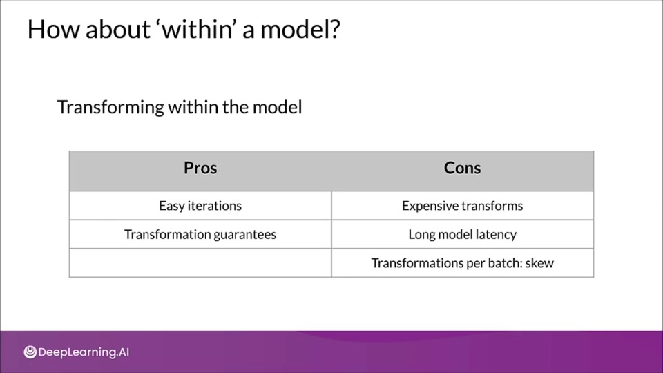
Feature Engineering within the model is limited to batch computations

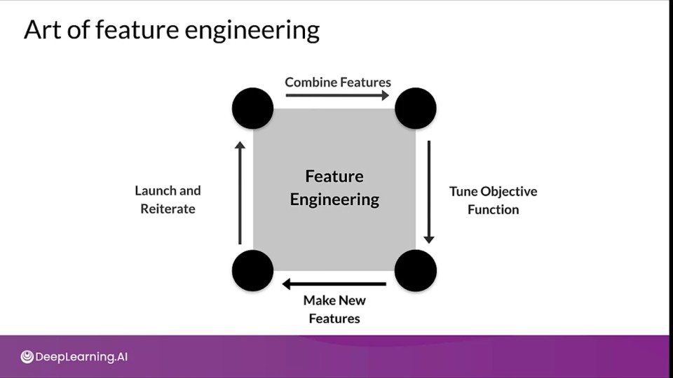
Art of feature engineering

Increases the model ability to learn while simultaneously reducing (if possible) the compute resources it requires.

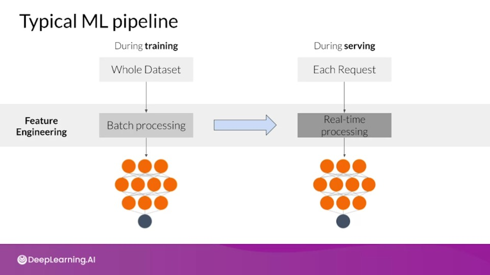
During serving we typically process each request individually, so it becomes important that we include global properties of our features, such as the $\sigma$ (standard deviation)

Preprocessing Operations

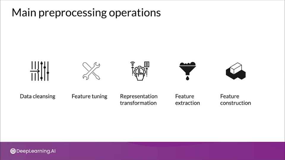
Data clearning to remove erroneous data.

Feature tuning like normalizing, scaling.

Representation transformation for better predictive signals

Feature Extraction / dimensionality reduction for more data representation.

Feature construction to create new features.

Mapping categorical values

Categorical values can be one-hot encoded if two nearby values are not more similar than two distant values, otherwise ordinal encoded.

Empirical knowledge of data will guide you further

Text: stemming, lemmatization, TF-IDF, n-grams, embedding lookup

Images - clipping, resizing, cropping, blur, canny filters, soble filters, photometric distortions

Key points

Data preprocessing: transforms raw data into a clean and training-ready dataset
Feature engineering maps:
- Raw data into feature vectors
- Integer values to floating-point values
- Normalizes numerical values
- String and categorical values to vectors of numeric values
- Data from one space into different space

Feature Engineering Techniques

Scaling

Converts values from their natural range into a prescribed range
- e.g., grayscale image pixel intensity scale is $[0, 255]$ usually rescaled to $[-1, 1]$

$$ x_\text{scaled} = \frac{(b-a)(x - x_{\min})}{x_{\max} - x_{\min}} + a \tag{$x$ $\isin$ [a, b]} $$

Normalization:

$$ x_\text{scaled} = \frac{x - x_{\min}}{x_{\max} - x_{\min}} \tag{$x$ $\isin$ [0, 1]} $$

Benefits
- Helps NN converge faster
- Do away with NaN errors during training
- For each feature, the model learn the right weights.

Standardization

Z-score relates the number of standard deviations away from the mean

$$ x_\text{std} = \frac{x - \mu}{\sigma} $$

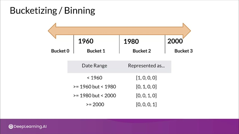
Bucketizing/ Binning

Other techniques

Dimensionality reduction in embeddings

Principle component analysis (PCA)
t-Distribute stochastic neighbor embedding (t-SNE)
uniform manifold approximation and projection (UMAP)

TensorFlow embedding projector

Intuitive explanation of high-dimensional data
Visualize & analyze

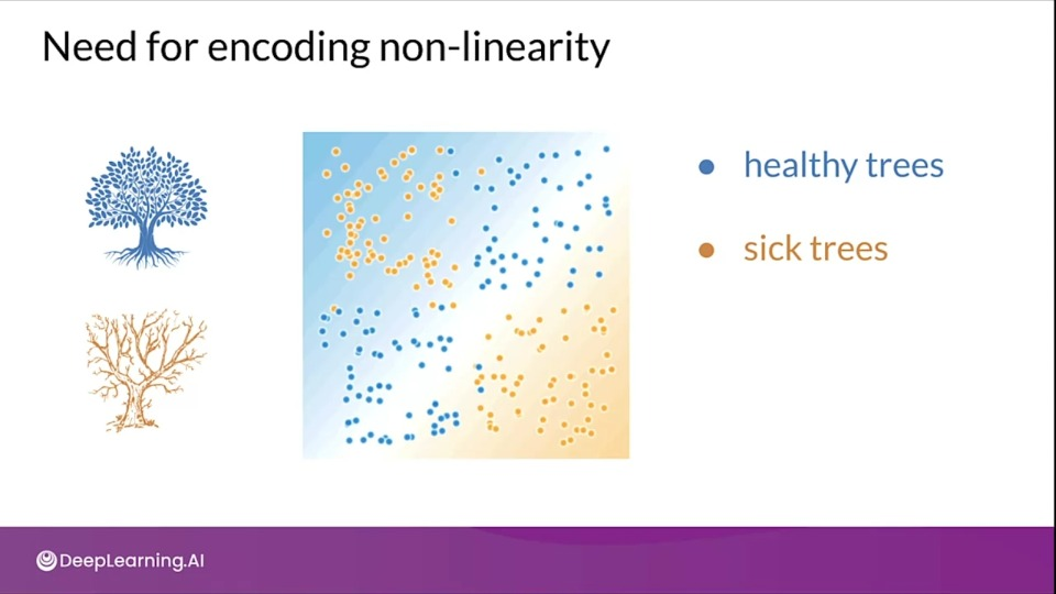
Feature Crosses

Combine multiple features together into a new feature
Encodes nonlinearity in the feature space, or encodes the same information in fewer features
$[A \times B]$ : multiplying the values of two features
$[A\times B\times C \times D \times E ]$: multiplying the values of 5 features
$[\text{Day of week, hour}] \rightarrow [\text{Hour of week}]$

Key points

Feature crossing: synthetic feature encoding nonlinearity in feature space
Feature coding: Transforming categorical to a continuous variable.

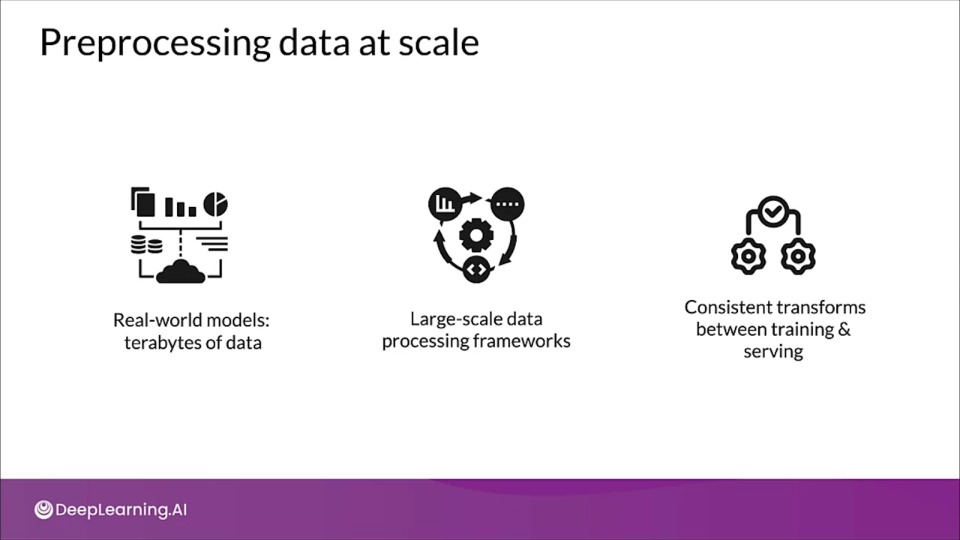
Feature Transformation at Scale — Preprocessing Data at Scale

To do feature transformation at scale we need ML pipeline to deploy our model with consistent and reproducible results.

Preprocessing at scale

Inconsistencies in feature engineering

Training & serving code paths are different
- Diverse deployment scenarios
  - Mobile (TensorFlow Lite)
  - Server (TensorFlow Serving)
  - Web (TensorFlow JS)
Risks of introducing training-serving skews
- Skews will lower the performance of your serving model

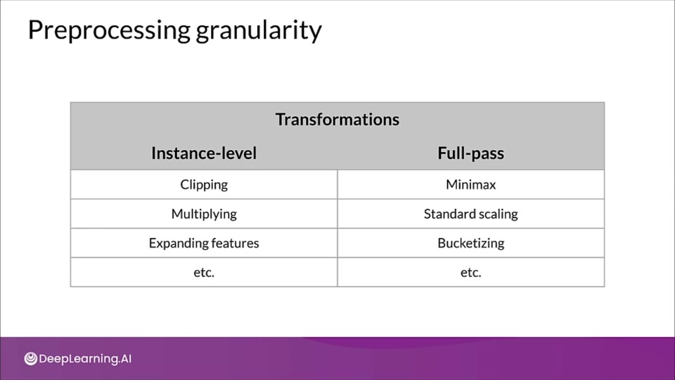
Preprocessing granularity

Applying Transformation per batch

For example, normalizing features by their average
Access to a single batch of data, not the full dataset
Ways to normalize per batch
- Normalize by average within a batch
- Precompute average and reuse it during normalization

Optimizing instance-level transformations

Indirectly affect training efficeincy
Typically accelerators sit idle while the CPUs transform
Solution:
- Prefetching transforms for better accelerator efficiency

Summarizing the challenges

Balancing predictive performance
Full-pass transformation on training data
Optimizing instance-level transformation for better training efficiency (GPUs, TPUs,...)

Key points

Inconsistent data affects the accuracy of the results
Need for scaled data processing frameworks to process large datasets in an efficient and distribute manner

TensorFlow Transform

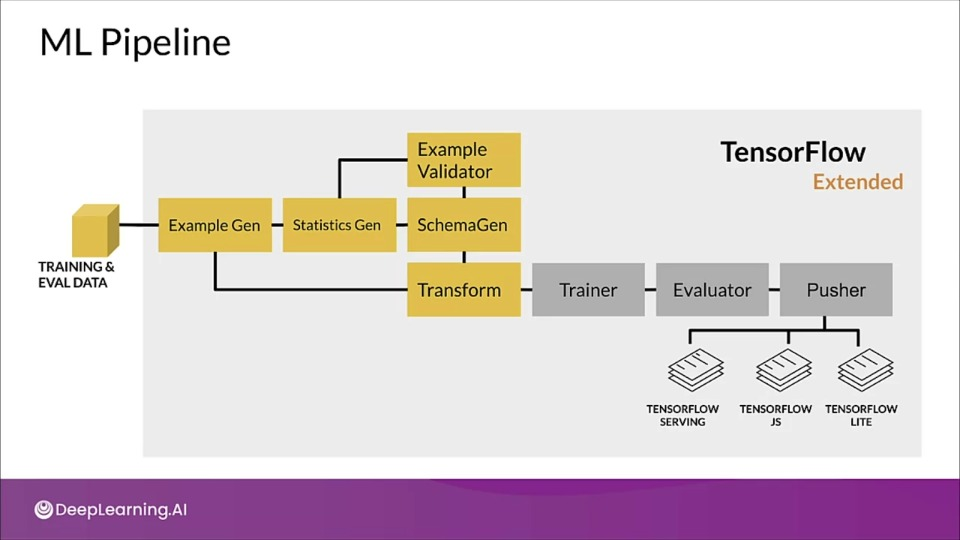
Example Gen: Generates Examples from the training & evaluation data

Statistics Gen: Generates Statistics

Schema Gen: Generates schema after ingesting statistics. This schema is then fed to:

Example validator: Takes schema and statistics and look for problems/anomalies in data
Transform: takes schema and dataset and do feature engineering

Trainer: Trains the model

Evaluator: Evaluates the result

Pusher: Pushes to wherever we want to serve our model.

tf.Transform: Going Deeper

tf.Transform Analyzers

Analyzers make a full pass over the dataset in order to collect constants that is required to do feature engineering. It also express the operations that we are going to do.

How Transform applies feature transformations

Benefits of using tf.Transform

Emitted tf.Graph holds all necessary constants and transformations
Focus on data preprocessing only at training time
Works in-line during both training and serving
No need for preprocessing code at serving time
Consistently applied transformations irrespective of deployment platform

Analyzers framework

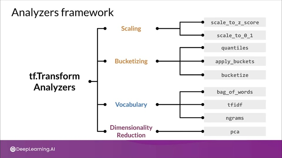
tf.Transform preprocessing_fn

def preprocessing_fn(inputs):
  ...
  for key in DENSE_FLOAT_FEATURE_KEYS:
    outputs[key] = tft.scale_to_z_score(inputs[key])

  for key in VOCAB_FEATURE_KEYS:
    outputs[key] = tft.vocabulary(inputs[key], vocab_filename=key)

  for jey in BUCKET_FEATURE_KEYS:
    outputs[key] = tft.bucketize(inputs[key], FEATURE_BUCKET_COUNT)

Commonly Used Imports

import tensorflow as tf
import apache_beam as beam
import apache_beam.io.iobase

import tensorflow_transform as tft
import tensorflow_transform.beam as tft_beam

Hello World with tf.Transform

Inspect data and prepare metadata

from tensorflow_transform.tf_metadata import (
    dataset_metadata, dataset_scehma)

# define sample data
raw_data = [
  {'x': 1, 'y': 1, 's': 'hello'},
  {'x': 2, 'y': 2, 's': 'world'},
  {'x': 3, 'y': 3, 's': 'hello'}
]

raw_data_metadata = dataset_metadata.DatasetMetadata(
  dataset_schema.from_feature_spec({
    'y': tf.io.FixedLenFeature([], tf.float32),
    'x': tf.io.FixedLenFeature([], tf.float32),
    's': tf.io.FixedLenFeature([], tf.string)
}))

Preprocessing data (Transform)

def preprocessing_fn(inputs):
  """Preproceess input columns into transformed columns"""
  x, y, s = inputs['x'], inputs['y'], inputs['s']
  x_centered = x - tft.mean(x)
  y_normalized = tft.scale_to_0_1(y)
  s_integerized = tft.compute_and_apply_vocabulary(s)
  # feature cross
  x_centered_times_y_normalized  (x_centered * y_normalized)
  return {
    'x_centered': x_centered,
    'y_normalized': y_normalized,
    's_integerized': s_integerized,
    'x_centered_times_y_normalized': x_centered_times_y_normalized,
  }

Running the pipeline

def main():
  with tft_beam.Context(temp_dir=tempfile.mkdtemp()):
    # Define a beam pipeline
    transformed_dataset, transform_fn = (
      (raw_data, raw_data_metadata) | tft_beam.AnalyzeAndTransformDataset(
          preprocessing_fn))

  transformed_data, transformed_metadata = transformed_datset
  print('\nRaw data:\n{}\n'.format(pprint.pformat(raw_data)))
  print('\Transformed data:\n{}'.format(pprint.pformat(tranformed_Data)))

if __name__ == '__main__':
        main()

Key points

tf.Transform allows the preprocessing of input data and creating features
tf.Transform allows defining pre-processing pipelines and their execution using large-scale data processing frameworks, like Apache Beam.
In a TFX pipeline, the Transform component implements feature engineering using TensorFlow Transform

Feature Selection — Feature Spaces

N dimensional space defined by your N features
Not including the target label

Feature space coverage

Train/Eval datasets should be representative of the serving dataset
- Same numerical ranges
- Same classes
- Similar characteristics for image data
- Similar vocabulary.

Ensure feature space coverage

Data affected by: seasonality, trend, drift
Serving data: new values in features and labels
Continuous monitoring, key for success!

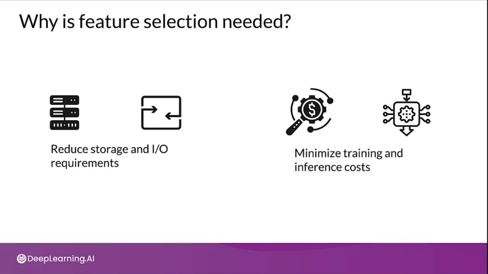
Feature Selection

Feature selection identifies the features that best represent the relationship between the features, and the target that we're trying to predict.
Remove features that don't influence the outcome
Reduce the size of the feature space
Reduces the resource requirements and model complexity

Unsupervised Feature selection methods

Feature-target variable relationship not considered
Removes redundant features (correlation)
- Two features that are highly correlated, you might need only one

Supervised feature selection

Uses features-target variable relationship
Selects those contributing the most

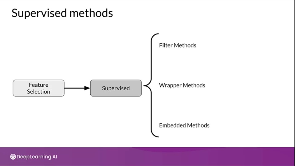
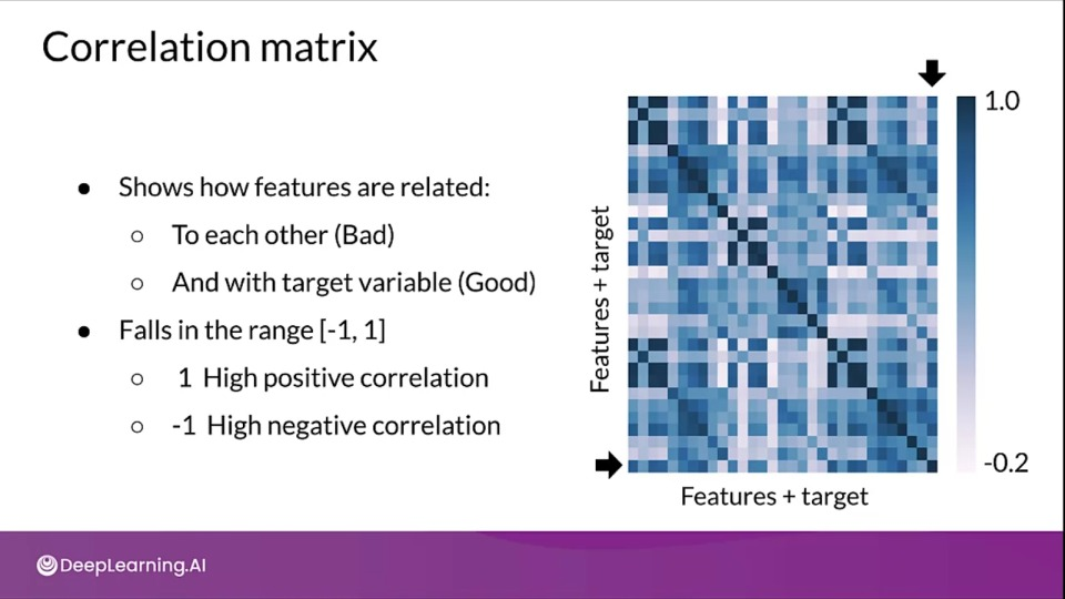
Filter methods

Correlated features are usually redunfant
- We remove them.
Filter methods suffer from inefficiencies as they need to look at all the possible feature subsets

Popular filter methods:

Pearson Correlation
- Between features, and between the features and the label
Univariate Feature Selection

Feature comparison statistical tests

Pearson's correlation: Linear relationships
Kendall Tau Rank Correlation Coefficient: Monotonic relationships & small sample size
Spearman's Rank Correlation Coefficient: Monotonic relationships

Other methods:

Pearson Correlation (numeric features - numeric target, exception: when target is 0/1 coded)
ANOVA f-test (numeric features - categorical target)
Chi-squared (categorical features - categorical target)
Mutual information

Determining correlation

# Pearson's correlation by default
cor = df.corr()

plt.figure(figsize=(20,20))
import seaborn as sns
sns.heatmap(cor, annot=True, cmap=plt.cm.PuBu)
plt.show()

Selecting Features

cor_target = abs(cor['diagnosis_int'])

# Selecting highly correlated features as potential features to eliminate
relavant_features = cor_target[cor_target > 0.2]

Univariate feature selection in Sklearn

Sklearn Univarite feature selection routines:

SelectKBest
SelectPercentile
GenericUnivariateSelect

Statistical tests available:

Regression: f__regression, mutual_info_regression
Classification: chi2 , f_classif, mutual_info_classif

`SelectKBest` implementation

def univariate_selection():
  X_train, X_test, y_train, y_test = train_test_split(X, y,
                  test_size=0.2, stratify=y, random_state=123)
  X_train_scaled = StandardScaler().fit_transform(X_train)
  X_test_scaled = StandardScaler().fit(X_train).transform(X_test)

  min_max_scaler = MinMaxScaler()
  scaled_X = min_max_scaler.fit_transform(X_train_scaled)

  selector = SelectKBest(chi2, k=20) # Use Chi-Squared test
  X_new = selector.fit_transform(scaled_X, y_train)
  feature_idx = selector.get_support()
  feature_names = df.drop("diagnosis_int", axis=1).columns[feature_idx]
  return feature_names

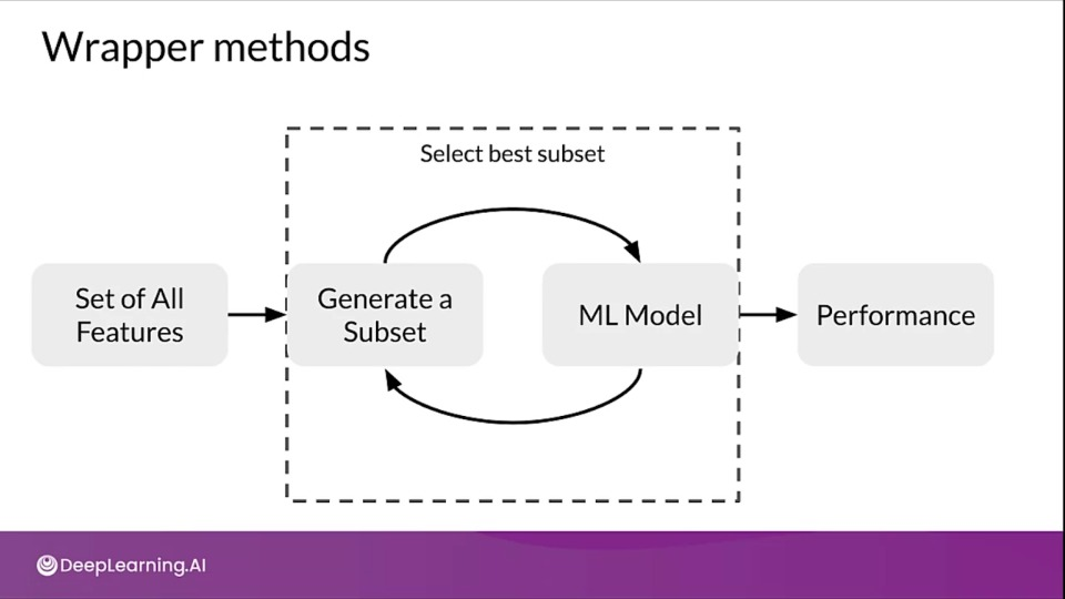
Wrapper Methods

It's a search method against the features that you have using a model as the measure of their effectiveness

Wrapper methods are based on greedy algorithm and this solutions are slow to compute.

Popular methods include:

Forward Selection
Backward Elimiation
Recursive Feature Elimination

Forward Selection

Iterative, greedy method
Starts with 1 feature
Evaluate model performance when adding each of the additional features, one at a time.
Add next feature that gives the best performance
Repeat until there is no improvement

Backward Elimination

Start with all features
Evaluate model performance when removing each of the included features, one at a time.
Remove next feature that gives the best performance
Repeat until there is no improvement

Recursive Feature Elimination (RFE)

Select a model to use for evaluating feature importance
Select the desired number of features
Fit the model
Rank features by importance
Discard least important features
Repeat until the desired number of features remains

def run_rfe():
  X_train, X_test, y_train, y_test = train_test_split(X, y,
                  test_size=0.2, stratify=y, random_state=123)

  X_train_scaled = StandardScaler().fit_transform(X_train)
  X_test_scaled = StandardScaler().fit(X_train).transform(X_test)

  model = RandomForestClassifier(criterion='entropy', random_state=47)
  rfe = RFE(model, 20)
  rfe = rfe.fit(X_train_scaled, y_train)
  feature_names = df.drop('diagnosis_int', axis=1).columns[rfe.get_support()]
  return feature_names

rfe_feature_names = run_rfe()

rfe_eval_df = evaluate_model_on_features(df[rfe_feature_names], y)

Embedded Methods

L1 regularization
Feature importance

Feature importance

Assigns scores for each feature in data
Discard features scores lower by feature importance

Feature importance with Sklearn

Feature Importance class is in-built in Tree Based Model (e.g., RandomForestClassifier)
Feature importance is available as a property feature_importances_
We can then use SelectFromModel to select features from the trained model based on assigned feature importances.

def feature_importances_from_tree_based_model_():
  X_train, X_test, y_train, y_test = train_test_split(X, y,
                  test_size=0.2, stratify=y, random_state=123)

  model = RandomForestClassifier()
  model = model.fitX_Train y_train)

  feat_importances = pd.Series(model.feature_importances_, index=X.columns)
  feat_importances.nlargest(10).plot(kind='barh')
  plt.show()
  return model

Select features based on importance

def select_features_from_model(model):
        model = SelectFromModel(model, prefit=True, threshold=0.012)
        feature_idx = df.drop("diagnosis_int", 1).columns[feature_idx]
        return feature_names

Tying together and evaluation

# Calcualte and plot feature importances
model = feature_importances_from_tree_based_model_()

# Select fearues based on feature importances
feature_imp_feature_names = select_features_from_model(model)

Week 2 References